Modeling Extreme Events: Time-Varying Extreme Tail Shape

Figures & data

Fig. 1 News impact curves.

The first element (left panel) and second element (right panel) of st in (7) is plotted against xt for different values of ξt and δt.

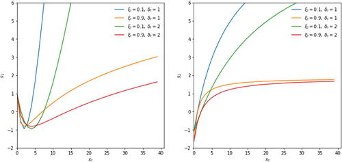
Fig. 2 Stationarity and moments regions.

Top row: the combinations of $a^{\xi }$ and $b^{\xi }$ that satisfy A2 (left panel), and (15) for p = 2 (middle panel) and p = 4 (right panel), for an increasing number of iterations $r\ge 1$. Bottom row: similar, but for combinations of $a^{\delta }$ and $b^{\delta }$ instead. Other deterministic parameters for each panel are fixed at their empirical estimates for S&P500 returns; see Section 4.1.

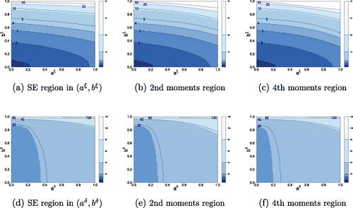
Fig. 3 Simulation results: an example.

Time series data is here generated as $y_t\sim$t$(0,{\sigma }_t,{\alpha }_t)$, where ${\alpha }_t^{-1}=0.5+0.3\hspace{0.17em}\sin \hspace{0.17em}(4\pi t/T)$ and ${\sigma }_t=1+0.5\hspace{0.17em}\sin \hspace{0.17em}(16\pi t/T)$. This is Path 3 in Section 3.1. Pseudo-true parameter values are reported in solid red. The four panels report estimates of ξt, δt, VaRt, and ESt, respectively. Median filtered values are plotted in solid black. The first two panels also indicate the lower 5% and upper 95% quantiles of the estimates (black dots). The time-varying threshold ${\widehat{\tau }}_t$ is estimated based on the recursive specification (10) in conjunction with the objective function (18).

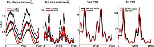
Table 1 RMSE outcomes for DGP1.

Model	GPD(τt)	GPD(${\widehat{\tau }}_t$)	GPD(${\widehat{\tau }}_t^{*}$)	t(τt)	t(${\widehat{\tau }}_t$)	t(${\widehat{\tau }}_t^{*}$)
	(infeasible)			(infeasible)
	RMSE ${\widehat{\xi }}_t$
(1)	0.000	0.000	0.000	0.000	0.000	0.000
	(0.000)	(0.000)	(0.000)	(0.000)	(0.000)	(0.000)
(2)	0.171	0.177	0.178	0.182	0.188	0.189
	(0.002)	(0.002)	(0.002)	(0.002)	(0.002)	(0.002)
(3)	0.182	0.188	0.189	0.190	0.197	0.197
	(0.002)	(0.002)	(0.002)	(0.002)	(0.002)	(0.002)
(4)	0.177	0.186	0.183	0.188	0.195	0.192
	(0.002)	(0.002)	(0.002)	(0.002)	(0.002)	(0.002)
	RMSE ${\widehat{\delta }}_t$
(1)	0.005	0.014	0.068	0.005	0.010	0.034
	(0.003)	(0.006)	(0.013)	(0.002)	(0.004)	(0.006)
(2)	1.646	1.774	1.753	0.580	0.589	0.588
	(0.034)	(0.040)	(0.036)	(0.013)	(0.012)	(0.013)
(3)	2.421	2.913	2.813	0.836	0.960	0.924
	(0.054)	(0.054)	(0.049)	(0.015)	(0.020)	(0.017)
(4)	2.608	2.904	2.844	0.925	0.970	0.964
	(0.057)	(0.059)	(0.059)	(0.020)	(0.020)	(0.022)

NOTE: Root mean squared error (RMSE) statistics for two different distributions (GPD and t, in columns) and for four different parameter paths for tail shape ξ_t and tail scale δ_t (paths (1)–(4), in rows). Thresholds τ_t, ${\widehat{\tau }}_t$, and ${\widehat{\tau }}_t^{*}$ denote, respectively, (i) the infeasible true time-varying threshold, (ii) the empirical quantile associated with an expanding window of observations $y_1,\dots ,y_t$, and (iii) the estimated conditional quantile using (18) and a suitably calibrated $a^{\tau }=0.25$ to speed up the computations. We consider 100 simulations for each DGP, and a time series of 25,000 observations in each simulation. Model performance is measured by the RMSE from the true ${\overline{\xi }}_t$ and ${\overline{\delta }}_t$ in each draw.

Table 2 Parameter estimates.

	First illustration		Second illustration
	S&P500	IBM	IT 5y yield		PT 5y yield
$a^{\xi }$	0.025	0.018	0.018	0.023	0.028	0.028
	(0.01)	(0.00)	(0.003)	(0.002)	(0.003)	(0.004)
	[0.00]	[0.00]	[0.000]	[0.000]	[0.000]	[0.000]
$a^{\delta }$	0.112	0.088	0.079	0.076	0.092	0.089
	(0.01)	(0.01)	(0.003)	(0.003)	(0.004)	(0.004)
	[0.00]	[0.00]	[0.000]	[0.000]	[0.000]	[0.000]
$b^{\xi }$	0.9993	0.9997	0.9997^a	0.9997^a	0.9997^a	0.9997^a
	(0.00)	(0.00)
	[0.00]	[0.00]
$b^{\delta }$	0.995	0.994	0.9997^a	0.9997^a	0.9997^a	0.9997^a
	(0.001)	(0.001)
	[0.00]	[0.00]
$c^{\xi }$				–7.696		–47.855
				(2.225)		(22.555)
				[0.001]		[0.034]
$c^{\delta }$				0.144		–10.782
				(0.737)		(4.323)
				[0.845]		[0.013]
λ	0	0	0.911	0.911	0.911	0.911
$a^{\tau }$	0.241	0.260	0.221	0.221	0.773	0.773
$b^{\tau }$	0.989	0.990	0.999	0.999	0.998	0.998
$c^{\tau }$			0.017	0.017	–0.141	–0.141
T	14,726	25,028	24,416	24,416	24,576	24,576
$T^{*}$	1495	2532	2448	2448	2490	2490
loglik	–22,028.4	–62,727.4	–80,535.8	–80,513.9	–196,068.0	–196,031.0
AIC	44,068.7	125,466.9	161,079.7	161,039.8	392,143.9	392,074.0
BIC	44,114.3	125,515.7	161,112.1	161,088.4	392,176.3	392,122.7

NOTE: Parameter estimates for the dynamic tail shape model. The second and third columns refer to the first application (equity log-returns of the S&P500 index and IBM stock). The estimation samples range from July 3, 1962 to December 31, 2020 for the S&P500 index, and from January 2, 1926 to December 31, 2020 for IBM stock. The remaining columns refer to the second application (changes in sovereign yields). Columns labeled IT 5y and PT 5y refer to yield changes for Italy and Portuguese five-year benchmark bonds sampled at the 15-min frequency. The estimation samples range from January 4, 2010, 9 a.m., to December 31, 2012, 5 p.m. For the second application, $b^{\xi }$ and $b^{\delta }$ are estimated indistinguishably different from, but still slightly below one. To be in line with theory, we fix the coefficients slightly below 1 at ${0.9997}^a$ for a = 1/32, such that at a daily (8 hr = 32 quarters) the coefficient is comparable to the highest IBM coefficient, $b^{\xi }$. Standard error estimates are in round brackets, p-values are in square brackets. Standard errors and p-values are based on a sandwich covariance matrix estimator for the first application, and on a bootstrap procedure for the second application.

Fig. 4 Filtered tail parameters for S&P500 (left) and IBM (right) log-returns.

Top panels: daily log-returns for the S&P500 index (left) and IBM common stock (right). Middle and bottom panels: filtered tail shape (ξt, middle) and tail scale (δt, bottom) parameters. The thresholds τt are reported at a 90% confidence level; Value-at-Risk (VaR) and Expected Shortfall (ES) are plotted at an extreme 99% confidence level (top panels). The thresholds τt, VaR, and ES are mirrored at the horizontal axis to correspond to log-returns (instead of percentage losses). The estimation samples range from July 3, 1962 to December 31, 2020 for the S&P500 index, and from January 2, 1926 to December 31, 2020 for the IBM stock. The reported samples range from July 3, 1962 to December 31, 2020.

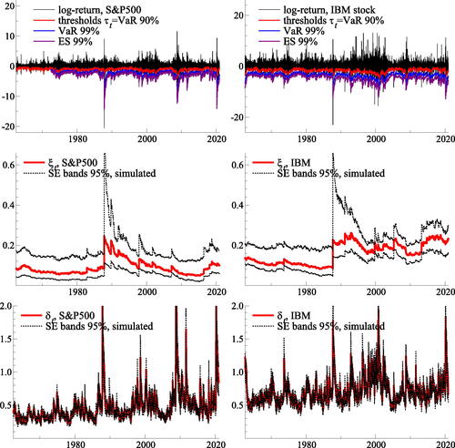
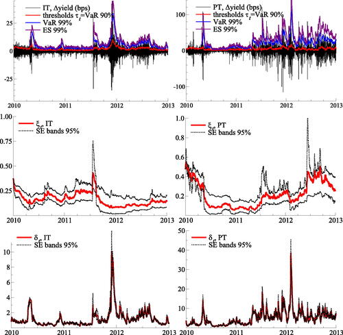
Fig. 5 The tail shape and tail scale estimates.

Top row: Five-year sovereign benchmark bond yields for Italy (IT, left column) and Portugal (PT, right column) between 2010 and 2012. Middle row: filtered tail shape (ξt) parameter. Bottom row: filtered tail scale (δt) parameter. Standard error bands are simulated at a 95% confidence level.