Estimating Posterior Sensitivities with Application to Structural Analysis of Bayesian Vector Autoregressions

Figures & data

Fig. 1 Comparing estimates of posterior mean derivatives (top panel) and their corresponding precision in terms of estimator standard deviations (bottom panel) obtained through the IPA on the x-axis and the LR on the y-axis. The findings are derived from 100 samples originating from DGP 2, using VAR(p) (p = 1, 2, 4) fitting under Minnesota shrinkage priors.

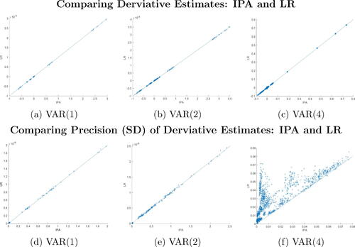
Fig. 2 Comparing estimates of posterior variance derivatives and their corresponding precision from IPA and FD under various bump sizes (1e-1, 1e-5, and 1e-17). Results are from fitting of a VAR(2) model under Minnesota shrinkage priors, using 100 samples drawn from DGP2.

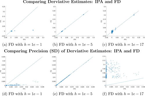
Fig. 3 IPA estimates of posterior mean and variance derivatives under Minnesota shrinkage priors for data simulated under DGP1 and DGP2. Presented estimates are for a VAR(2) or VAR(4) model for the sensitivities of posterior means and variances of VAR coefficients in the first equation with respect to the corresponding prior means and variances.

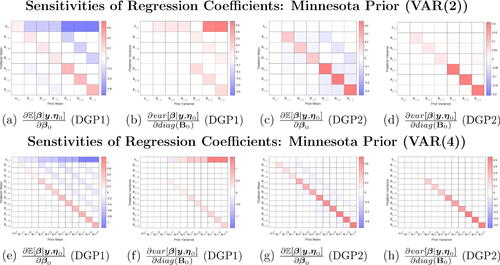
Fig. 4 IPA estimates of posterior mean and variance derivatives under the Uninformative prior for data simulated under DGP1 and DGP2. Presented estimates are sensitivities of posterior means and variances of VAR coefficients in the first equation with respect to the corresponding prior means and variances for inference under a VAR(2) model.

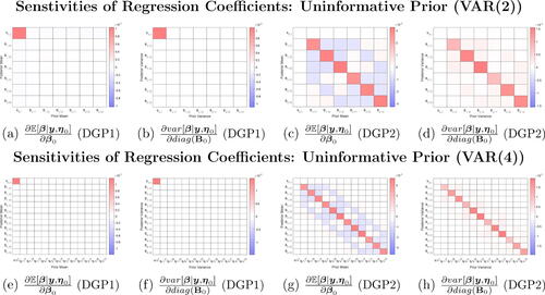
Fig. 5 IPA estimates of posterior forecast error variance decomposition $\mathbf{\text{FEV}}{\mathbf{D}}_{2,1,t}$ ($t=0,1,\dots ,16$) with respect to both prior means and prior variances of VAR coefficients in the first equation under Minnesota shrinkage prior for data simulated from DGP1 and DGP2.

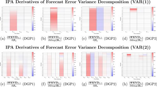
Fig. 6 IPA and “Relative” IPA estimates of posterior ${\mathit{\text{IRF}}}_{2,1,t}$ ($t=0,1,\dots ,16$) with respect to prior means and prior variances of VAR coefficients in the first equation under Minnesota shrinkage prior for data simulated from DGP1 and DGP2.

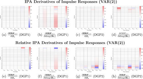
Fig. 7 Mean derivatives of model coefficients from all three equations with respect to the prior means $\frac{\partial \widehat{\mathit{\beta }}}{\partial {\mathit{\beta }}_0}$ (top panels) and prior variances $\frac{\partial \widehat{\mathit{\beta }}}{\partial \mathit{\text{diag}}({\mathbf{B}}_0)}$ (bottom panels) of prior parameters in the GDP equation.

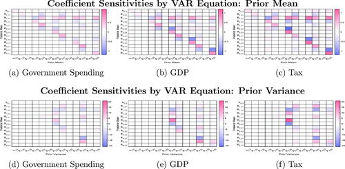
Fig. 8 Heatmaps of derivative estimates (in absolute values) of largest eigenvalue λ₁ with respect to the prior mean and variance parameters. The three rows are derivatives of λ₁ with respects to prior parameters associated with the Government spending, GDP, and Tax equations, respectively.

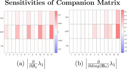
Fig. 9 Heatmaps of derivative estimates of the IRF and FEVD of log GDP at 20 quarters after the spending shock with respect to the prior mean parameters and variance parameters. The three rows are derivatives with respects to prior parameters associated with the Government spending, GDP and Tax equations, respectively.

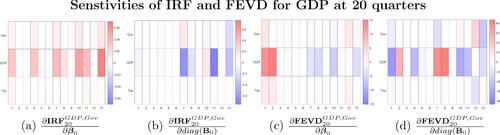
Fig. 10 IPA-based GDP response changes (${\widehat{\mathit{\text{IRF}}}}^{\mathit{\text{GDP}},\mathit{\text{Gov}}}({\mathit{\eta }}_0+\delta )$ under various perturbations $(\delta =1e-03,\delta =3e-03)$ of prior parameter settings (prior mean and variance parameters, prior mean parameters, prior variance parameters) under RW prior.

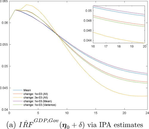
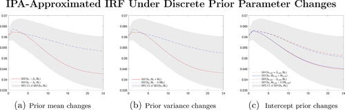
Fig. 11 Approximated change of GDP response to spending shock, ${\widehat{\mathbf{\text{IRF}}}}^{\mathit{\text{GDP}},\mathit{\text{Gov}}}$, under relative changes in prior mean and variances based on AD derivatives/first order Taylor series expansion compared to 68% IRF interval under initial prior setting.

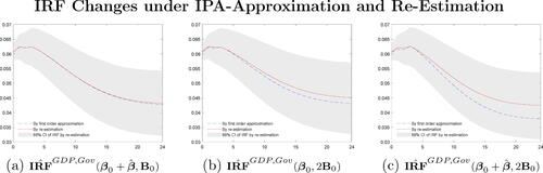
Fig. 12 Approximated change of GDP response to spending shock, ${\widehat{\mathbf{\text{IRF}}}}^{\mathit{\text{GDP}},\mathit{\text{Gov}}}$, under relative changes in prior mean and variances based on AD derivatives/first order Taylor series expansion compared to 68% IRF interval under initial prior setting. For changes in the intercept prior both mean and variances are changed.