Figures & data
Figure 1. Organization of rest-activity behavior and sleep times. The left two columns display the double-plotted raster actograms derived from Fitbit “steps” data over the course of the study month showing the rest-activity behavior of a “regular sleeper” (left) and an “irregular sleeper” (middle). Amplitude (number of “steps” per minute) is plotted on the vertical axis, whereas “Time of day” in hours is plotted on the horizontal axis. The right-most panel (“#sleep episodes”) displays the timing of habitual sleep occurring at multiple clock times of the day and night derived from Fitbit sleep onset times in a double plotted raster format for all participants (n = 89). The vertical axis displays all individuals’ data sets, whereas the horizontal axis displays “Sleep onset time” in hours. The number of sleep episodes per 30 minutes is displayed beneath and is color-coded to highlight density of sleep onset occurrence
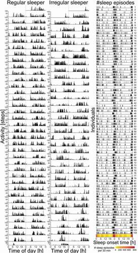
Figure 2. Distribution of morningness – eveningness scores (n = 85) derived from the German version of the reduced Horne-Östberg Morningness-Eveningness Questionnaire (rMEQ) (Randler Citation2013). The rMEQ scores are plotted on the horizontal axis and their colors correspond to the rMEQ-derived chronotypes labeled beneath. The number (“Count”) of individuals per score is plotted on the vertical axis. The dashed vertical lines delineate the Evening Types (rMEQ score ≤ 11; n = 20), Intermediate Types (11 < rMEQ score < 18; n = 45) and Morning Types (rMEQ score ≥ 18; n = 20)
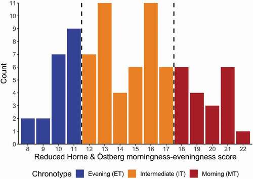
Table 1. Demographic characteristics
Figure 3. Variations in the occurrence and internal organization of sleep across the day derived from Fitbit Charge 2TM sleep data. Morning Type (n = 20; red dots and lines), Intermediate Type (n = 45; orange dots and lines) and Evening Type (n = 20; blue dots and lines) data are plotted for variables ‘Sleep Duration’ (left) and ‘Wake After Sleep Onset’ (right). All plots have time of sleep onset in hours as the horizontal axis. Panel A displays individual data points, their averages (curves), as well as peak and nadir (circles on curves). The vertical axis of ‘Sleep Duration’ displays time in hours, whereas this axis shows percentage of sleep episode for variable ‘Wake After Sleep Onset.’ Confidence intervals for maxima and minima are displayed horizontally beneath and vertically to the right of the figures of panel A (color-coded bars match the respective chronotype). Panels B, C and D display non-linear diurnal modulations over time of day and 95% simultaneous confidence intervals (shaded area around curves); the vertical axes are in arbitrary units; gray bars on top of panels B and C indicate values that differ significantly from intercept (dashed line). Panel B shows data for the entire sample, whereas panel C displays data per chronotype. Panel D shows the differences between the chronotypes, such as indicated on the right; the gray bars on top of the panels indicate the times where the waveshapes differed significantly from one another
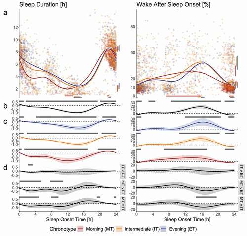
Figure 4. Variations in the occurrence and internal organization of REM sleep across the day derived from Fitbit Charge 2TM sleep data. Morning Type (n = 20; red dots and lines), Intermediate Type (n = 45; orange dots and lines) and Evening Type (n = 20; blue dots and lines) data are plotted for variables ‘REM Sleep Percentage in first NREM-REM cycle’ (REM%; left) and ‘REM Sleep Latency’ (RL; right). All plots have time of sleep onset in hours as the horizontal axis. Panel A displays individual data points, their averages (curves), as well as peak and nadir (circles on curves). The vertical axis of ‘REM%’ displays time as a percentage of sleep episode, whereas for variable ‘RL’ the vertical axis shows time in hours. Confidence intervals for maxima and minima are displayed horizontally beneath and vertically to the right of the figures of panel A (color-coded bars match the respective chronotype). Panels B, C and D display non-linear diurnal modulations over time of day and simultaneous confidence intervals (shaded area around curves); the vertical axes are in arbitrary units; gray bars on top of panels B and C indicate that values differ significantly from intercept (dashed line). Panel B shows data for the entire sample, whereas panel C displays data per chronotype. Panel D shows the differences between the chronotypes, such as indicated on the right; the gray bars on top of the panels indicate the times where the waveshapes differed significantly from one another
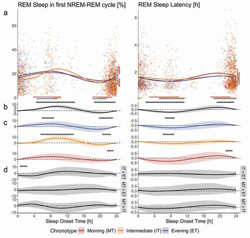
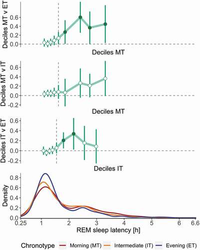
Figure 5. Density distribution of REM sleep latencies in morning (MT, n = 20), intermediate (IT, n = 45) and evening type (ET, n = 20) study participants. The top three panels display the decile difference among MT, IT and ET. Circles represent average decile differences, whereas whiskers show bootstrapped confidence intervals corrected for multiple comparison. The dashed vertical line in the top two panels represents the median in MT; in the 3rd panel it represents the median in IT. The bottom panel describes the density functions of RL by chronotype (MT = red, IT = orange, ET = blue). The horizontal axis is shared by all panels and shows RL in hours. Compared to ET, the RL distributions in IT and MT display more weight in potential missed first REM sleep episodes (RL > 2 h)