Figures & data
Figure 1. Left panel: Technical design for PAT measurement: ECG for detection of the Q- or R-wave, PPG for detection of the peripheral volume pulse. Recorder: data collection, AD-conversion, data pre-processing, storage. Right panel: PAT-Detection from ECG and PPG, here from the start of Q-wave to the beginning of PPG signal rise. In the literature, several other points in the physiological signals, such as the R-wave peak or the steepest increase of the PPG signal have been used for PAT detection. This results in different PAT values.
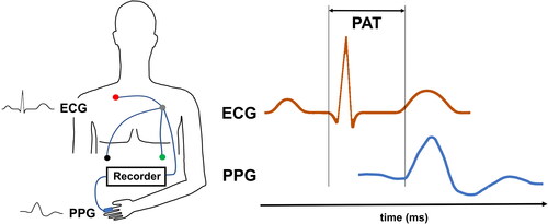
Table 1. Recent studies focussing on improving cuffless BP measurements.
Figure 2. Graphical display of PAT, PEP and PTT. PAT and PTT may vary depending on the starting point, for PAT see also . PAT is the time between electrical heart excitation (ECG (1)) and the arrival of the subsequent pulse wave in the periphery (PPG (3)). PTT is the time delay between the onset of a central mechanical wave (here pressure pulse in the aorta (2)) and the arrival of the same pulse wave in the periphery (PPG (3)). PEP is the time between electrical heart excitation (ECG (1)) and the onset of a central mechanical wave (Aorta (2)).
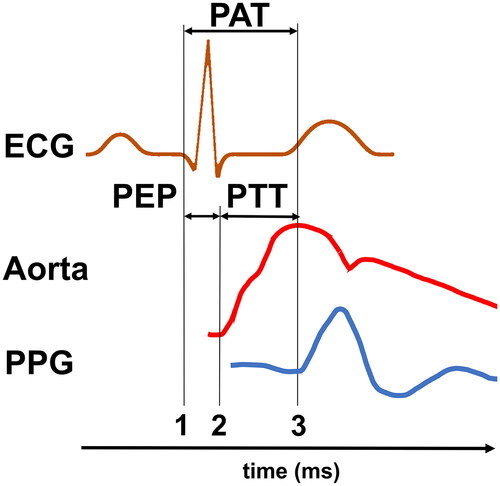
Figure 3. Upper panel: Calculation of PIR as the difference between peak (IP) and valley intensity (Iv) of the PPG. Lower panel: First deviation of the PPG signal (dPPG). dPIR is the difference between the peak- (dIp) and the valley intensity (dIv).
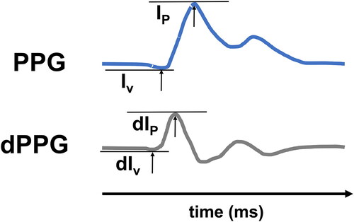
Figure 4. HPSR (left panel) of a time series of instantaneous HR (right panel). LF: power in the range between 0.05 and <0.2 Hz, HF: power in the range between 0.2 and 0.5 Hz.
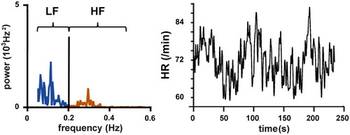
Table 2. Device performances of already tested for 24-h usage and experimental cuffless BP measurement devices.
Figure 5. Example structure of a Regression Tree. Each layer splits the data based on decision boundaries regarding a single input feature. As an illustration, the first layer splits the data into female and male subsets. The second layer splits the data based on another feature. Regression Trees can have unlimited amounts of decision-layers. The final layer consists of leaves with transfer functions which are used to calculate the final output.
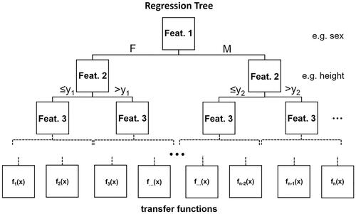
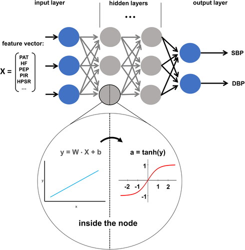
Figure 6. Schematic structure of Deep Learning architecture. Input features are fed into the model as a vector and passed into the hidden layers. Hidden layer nodes take the inputs and run them through two calculations (inside the node). First, a multilinear equation takes a weight vector (W), the input vector (X), and a bias term (b) to calculate a temporary variable (y). This variable is then fed into a non-linear activation function (e.g. tanh) to calculate the node’s output (a). All nodes within a layer pass their output to all nodes in the following layer (arrows) which stack them into a vector and treat them as their input vector. The final hidden layer passes its activations (a) into the output layer, which in this case has two nodes (for SBP and DBP). Nodes in the output layer do not have an activation function and output the result of their linear function (y). The model is trained by optimising each node’s W and b to minimise the difference between a ground truth presented by the training dataset and the models corresponding predictions.