Publication Cover
Australian Journal of Earth Sciences
An International Geoscience Journal of the Geological Society of Australia
Volume 54, 2007 - Issue 1
682
Views
5
CrossRef citations to date
0
Altmetric
Original Articles

Numerical modelling of the western Hodgkinson Province, northeast Queensland: implications for gold mineralisation

, , &
Pages 27-47 | Received 08 Jul 2005, Accepted 28 Jul 2006, Published online: 15 Jan 2007

Figures & data

Figure 1 General geology of the Hodgkinson Province. The Palmerville Fault forms the bounding structure at the western margin of the province that accommodated major basin extension and inversion during the Palaeozoic (Vos et al. in press).
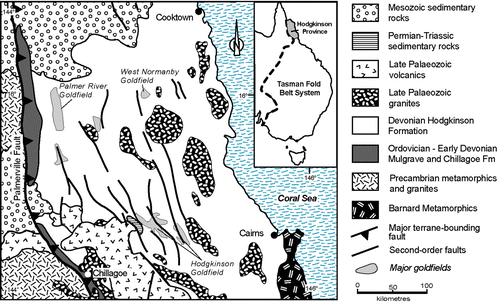
Figure 1 General geology of the Hodgkinson Province. The Palmerville Fault forms the bounding structure at the western margin of the province that accommodated major basin extension and inversion during the Palaeozoic (Vos et al. in press).

Figure 2 Overview of the Palaeozoic geological evolution of the Hodgkinson Province, including tectonic, metallogenic, magmatic and sedimentary events, indicating the time frame considered for modelling in this study (after Vos & Bierlein Citation2006).
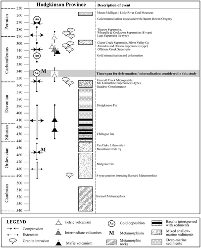
Figure 2 Overview of the Palaeozoic geological evolution of the Hodgkinson Province, including tectonic, metallogenic, magmatic and sedimentary events, indicating the time frame considered for modelling in this study (after Vos & Bierlein Citation2006).

Figure 3 Overall model architecture representing a block of crust 50 km wide, 50 km long and 5 km deep. (a) Base architecture with two lithologies and three through-going faults showing the model setup in plan view (top) and cross-section (bottom). (b) Variations on the base architecture with three lithologies and no faults (top) and three lithologies, two through-going faults and a fault segment covering half the blocks length (bottom).
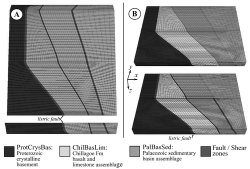
Figure 3 Overall model architecture representing a block of crust 50 km wide, 50 km long and 5 km deep. (a) Base architecture with two lithologies and three through-going faults showing the model setup in plan view (top) and cross-section (bottom). (b) Variations on the base architecture with three lithologies and no faults (top) and three lithologies, two through-going faults and a fault segment covering half the blocks length (bottom).

Table 1  Overview of model architectures, with varying number of faults, lithologies and pore pressure.

Table 2  Rock properties for lithologies used in model setups.

Figure 4 (a) Extent of bounding box (buffer zone) surrounding the model architecture (internal model box) to minimise boundary effects that may result from boundary conditions as discussed in text. This bounding box allows fluids to flow through the internal box (which represents the region of interest) without actually flowing out of the entire model. Note that the first 5 km of the external bounding box have been made transparent, so the start of the internal model box is visible, surrounded by the buffer zone on both sides and along the top. (b) Schematic pore-pressure vs depth diagram: Line A represents one of the two initial (prior to model equilibration) pore pressure conditions imposed upon the models (0.5×lithostatic pore fluid pressure). Curve 1 indicates the post-equilibration fluid-pressure conditions where the pore pressure has equilibrated to a hydrostatic gradient, but at supra-hydrostatic pressures. Curve 2 is indicative of pore pressures after injection of fluids at the base of the model (in those models which incorporate fluid injection).
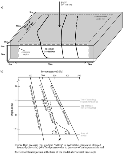
Figure 4 (a) Extent of bounding box (buffer zone) surrounding the model architecture (internal model box) to minimise boundary effects that may result from boundary conditions as discussed in text. This bounding box allows fluids to flow through the internal box (which represents the region of interest) without actually flowing out of the entire model. Note that the first 5 km of the external bounding box have been made transparent, so the start of the internal model box is visible, surrounded by the buffer zone on both sides and along the top. (b) Schematic pore-pressure vs depth diagram: Line A represents one of the two initial (prior to model equilibration) pore pressure conditions imposed upon the models (0.5×lithostatic pore fluid pressure). Curve 1 indicates the post-equilibration fluid-pressure conditions where the pore pressure has equilibrated to a hydrostatic gradient, but at supra-hydrostatic pressures. Curve 2 is indicative of pore pressures after injection of fluids at the base of the model (in those models which incorporate fluid injection).

Table 3  Modes of deformation used in model runs.

Figure 5 Model deformation conditions (plan view). (a) Plane strain: model is subject to 10% shortening along the x-axis. (b) Transpression: model is subject to 5% sinistral strike-slip deformation along the z-axis, in addition to 10% shortening along the x-axis. External (fat) arrows indicate relative magnitudes of x and z velocities applied to model boundaries; internal (finer) arrows indicate the magnitude and direction of forces working on the cell mesh. The grey-shaded area indicates central focus area towards which deformation forces are directed.
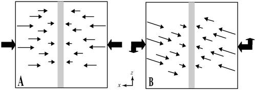
Figure 5 Model deformation conditions (plan view). (a) Plane strain: model is subject to 10% shortening along the x-axis. (b) Transpression: model is subject to 5% sinistral strike-slip deformation along the z-axis, in addition to 10% shortening along the x-axis. External (fat) arrows indicate relative magnitudes of x and z velocities applied to model boundaries; internal (finer) arrows indicate the magnitude and direction of forces working on the cell mesh. The grey-shaded area indicates central focus area towards which deformation forces are directed.

Table 4  Overview of completed model runs indicating model setup (see ) and deformation modes used (see ).

Figure 6 3D representation of cumulative shear-strain distribution after 9% shortening: (a) plane strain, listric fault (Model Run 1); (b) transpression, listric fault (Model Run 2); (c) plane strain, planar fault (Model Run 1); (d) transpression, planar fault (Model Run 2). Model run numbers relate to .
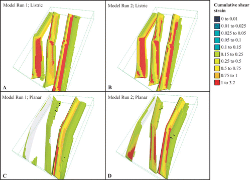
Figure 6 3D representation of cumulative shear-strain distribution after 9% shortening: (a) plane strain, listric fault (Model Run 1); (b) transpression, listric fault (Model Run 2); (c) plane strain, planar fault (Model Run 1); (d) transpression, planar fault (Model Run 2). Model run numbers relate to Table 4.

Figure 7 3D representation of cumulative distribution of dilation (percentage volume increase) after 9% shortening: (a) plane strain, listric fault (Model 1); (b) transpression, listric fault (Model 2); (c) plane strain, planar fault (Model 1); (d) transpression, planar fault (Model 2). Model run numbers relate to . Negative values indicate percentage volume loss/compaction.
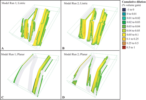
Figure 7 3D representation of cumulative distribution of dilation (percentage volume increase) after 9% shortening: (a) plane strain, listric fault (Model 1); (b) transpression, listric fault (Model 2); (c) plane strain, planar fault (Model 1); (d) transpression, planar fault (Model 2). Model run numbers relate to Table 4. Negative values indicate percentage volume loss/compaction.

Figure 8 3D representation of cumulative shear strain distribution after 9% shortening in a listric fault scenario: (a) two lithologies, plane strain, with increased initial pore fluid pressure (0.8×lithostatic, Model Run 3); (b) two lithologies, transpression, with increased initial pore fluid pressure (0.8×lithostatic, Model Run 4); (c) three lithologies, plane strain (Model Run 5); (d) three lithologies, transpression (Model Run 6); (e) three lithologies, plane strain, with cell permeability increasing at yield (Model Run 7); (f) three lithologies, transpression, with cell permeability increasing at yield (Model Run 8). Model run numbers relate to .
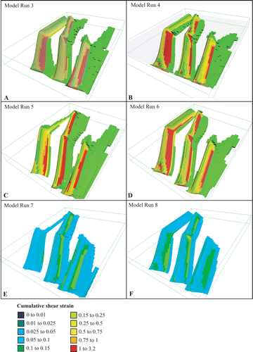
Figure 8 3D representation of cumulative shear strain distribution after 9% shortening in a listric fault scenario: (a) two lithologies, plane strain, with increased initial pore fluid pressure (0.8×lithostatic, Model Run 3); (b) two lithologies, transpression, with increased initial pore fluid pressure (0.8×lithostatic, Model Run 4); (c) three lithologies, plane strain (Model Run 5); (d) three lithologies, transpression (Model Run 6); (e) three lithologies, plane strain, with cell permeability increasing at yield (Model Run 7); (f) three lithologies, transpression, with cell permeability increasing at yield (Model Run 8). Model run numbers relate to Table 4.

Figure 9 Mohr – Coulomb diagram illustrating the effect of dilation leading to fluid pressure decrease after cell failure.
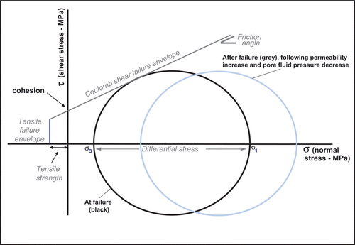
Figure 9 Mohr – Coulomb diagram illustrating the effect of dilation leading to fluid pressure decrease after cell failure.

Figure 10 3D representation of instantaneous fluid-flow vectors after 9% shortening indicating magnitude of Darcian fluid flow (m/s) for model scenarios as described in . The majority of fluid flow vectors overlap with faults. Black arrows indicate the representative direction of fluid flow (see text for discussion).
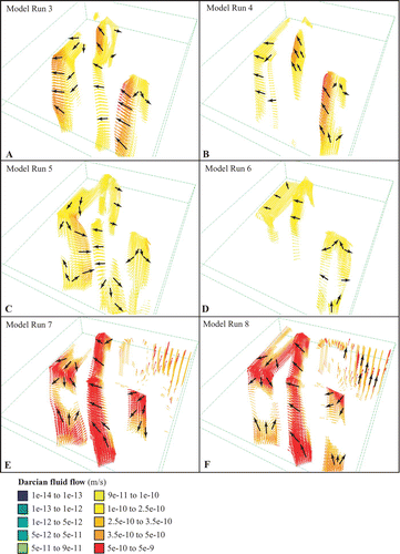
Figure 10 3D representation of instantaneous fluid-flow vectors after 9% shortening indicating magnitude of Darcian fluid flow (m/s) for model scenarios as described in Figure 8. The majority of fluid flow vectors overlap with faults. Black arrows indicate the representative direction of fluid flow (see text for discussion).

Figure 11 View of base of various model architectures with local fluid injection indicated by dashed lines (see text for discussion): (a) fluid flux into the sedimentary assemblage; (b) fluid flux into the central and eastern faults; (c) fluid flux into the sedimentary assemblage in a no-fault model architecture.
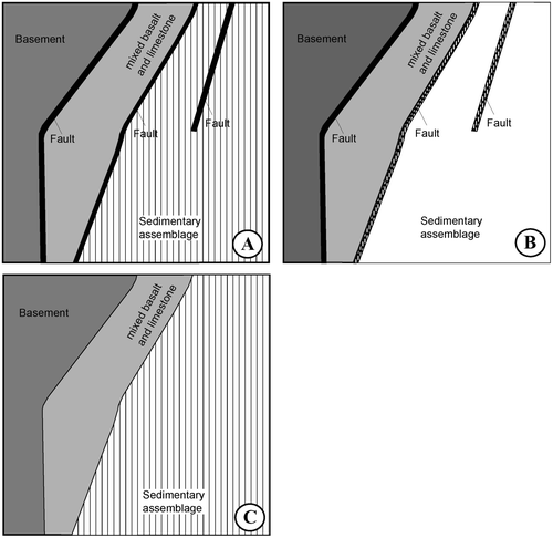
Figure 11 View of base of various model architectures with local fluid injection indicated by dashed lines (see text for discussion): (a) fluid flux into the sedimentary assemblage; (b) fluid flux into the central and eastern faults; (c) fluid flux into the sedimentary assemblage in a no-fault model architecture.

Figure 12 3D representation of cumulative shear strain distribution after 9% shortening in a listric fault scenario with fluid injection over specified regions at the base of the model: (a) plane strain, fluid injected into sedimentary assemblage (Model Run 9); (b) transpression, fluid injected into sedimentary assemblage (Model Run 10); (c) plane strain, fluid injected into central and eastern faults (Model Run 17); (d) transpression, fluid injected into central and eastern faults (Model Run 18); (e) plane strain, fluid injected into sedimentary assemblage and faults absent (Model Run 13); (f) transpression, fluid injected into sedimentary assemblage and faults absent (Model Run 14). Model run numbers relate to .
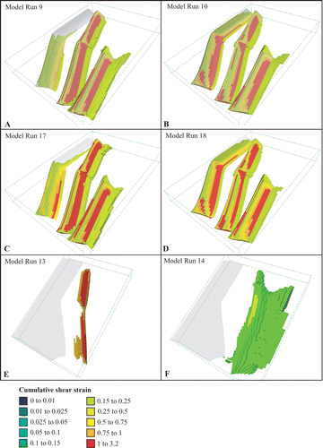
Figure 12 3D representation of cumulative shear strain distribution after 9% shortening in a listric fault scenario with fluid injection over specified regions at the base of the model: (a) plane strain, fluid injected into sedimentary assemblage (Model Run 9); (b) transpression, fluid injected into sedimentary assemblage (Model Run 10); (c) plane strain, fluid injected into central and eastern faults (Model Run 17); (d) transpression, fluid injected into central and eastern faults (Model Run 18); (e) plane strain, fluid injected into sedimentary assemblage and faults absent (Model Run 13); (f) transpression, fluid injected into sedimentary assemblage and faults absent (Model Run 14). Model run numbers relate to Table 4.

Figure 13 3D representation of instantaneous fluid-flow vectors after 9% shortening indicating the magnitude of Darcian fluid flow (m/s) for model scenarios as described in . Fluid-flow vectors overlap with faults in c and d. Black arrows are added to indicate the representative direction of fluid flow (see text for discussion).
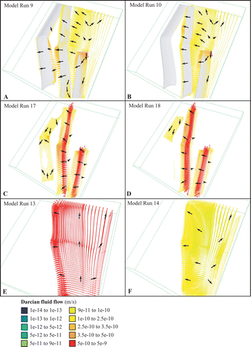
Figure 13 3D representation of instantaneous fluid-flow vectors after 9% shortening indicating the magnitude of Darcian fluid flow (m/s) for model scenarios as described in Figure 12. Fluid-flow vectors overlap with faults in c and d. Black arrows are added to indicate the representative direction of fluid flow (see text for discussion).

Reprints and Corporate Permissions

Please note: Selecting permissions does not provide access to the full text of the article, please see our help page How do I view content?

To request a reprint or corporate permissions for this article, please click on the relevant link below:

Academic Permissions

Please note: Selecting permissions does not provide access to the full text of the article, please see our help page How do I view content?

Obtain permissions instantly via Rightslink by clicking on the button below:

If you are unable to obtain permissions via Rightslink, please complete and submit this Permissions form. For more information, please visit our Permissions help page.