Figures & data
Figure 1 (a) Forces acting along the Indo-Australian Plate. H, Himalaya; S, Sumatra Trench; J, Java Trench; B, Banda Arc; NG, New Guinea; SM, Solomon Trench; NH, New Hebrides; TK, Tonga–Kermadec Trench; NZ, New Zealand; SNZ, south of New Zealand; MOR, mid-ocean ridge; LHR, Lord Howe Rise; cb, collisional boundary; sz, subduction zone; ia, island arc. (b) Stress field within the Australian continent. Stress trajectories as predicted by a thin elastic-plate model driven by forces originating along the plate compressional boundaries, superimposed on averaged stress orientation estimates from large earthquakes and borehole data (from Reynolds et al. Citation2002).
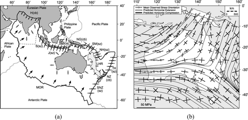
Figure 2 (a) Present-day topography averaged over 1° × 1° cells. 1, southeastern Highlands; 2, Mt Lofty/Flinders Ranges; 3, southwestern Yilgarn Craton; 4, Albany–Fraser Province; 5, central Australian basins; 6, Canning Basin; 7, southeastern Queensland Highlands; 8, Eromanga Basin; 9, Murray Basin; 10, Gawler Craton; DF, Darling Fault. (b) Distribution of seismicity within the Australian continent as observed in the period 1950–2007.
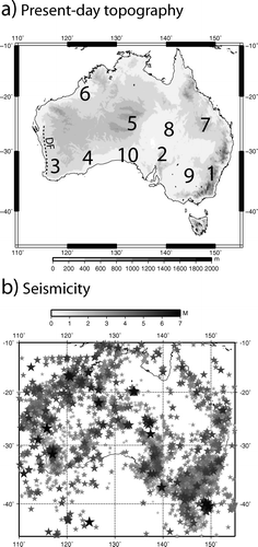
Figure 3 (a–c) Seismic strain rate as predicted from the distribution and magnitude of earthquakes observed over the 1970–2007 period assuming: (a) a maximum earthquake magnitude, M max of 7, aftershocks removed and a 2° × 2° binning of the data; (b) without removing the aftershocks; and (c) a 1° × 1° binning of the data. (d, e) Computed a and b values corresponding to (a). (f) Earthquake distribution, i.e. number of events in each cell.
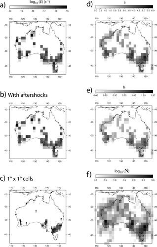
Figure 4 (a) Present-day topography. (b) Filtered topography, i.e. maximum topography in 2° × 2° bins. (c, d) Predicted seismic uplift obtained by extrapolating current strain rate over a 10 Ma period and assuming (c) local isostasy and (d) flexural isostasy.
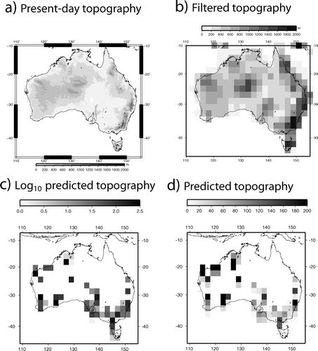
Figure 5 Predicted seismic uplift obtained under the assumption of regional, flexural isostasy. (a) and (b) represent the same results; they differ by the scale used to highlight different aspects (low and high amplitude) of the computed topography.
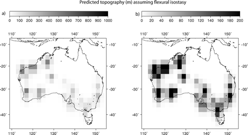
Figure 6 (a) Horizontal cross-section at 100 km depth through the deviation in seismic velocity from a mean reference velocity derived from the SKIPPY data. Darkest red areas correspond to a relative deviation of –8%; darkest blue areas correspond to a relative deviation of 8% (Fishwick et al. Citation2005). (b) Computed seismic strain rate for comparison. Question marks indicate regions where there is no match between deformation and present-day topography; V-symbols in indicate where this match is present.
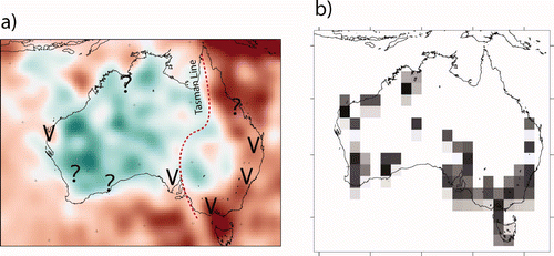
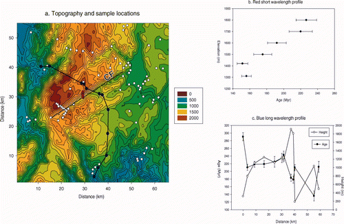
Figure 7 (a) Location of samples for fission-track apatite ages in the Snowy Mountain area of the southeastern Highlands (circles) superimposed on the topography. Location of red and blue profiles are also shown. Dotted line (CF) is trace of Crackenback Fault. (b) Age vs elevation along the red profile. (c) Age and elevation along the blue profile from southeast to northwest.