Characterisation of geological thin layer by borehole radar

Figures & data

Figure 1. Schematic illustration of ray paths of crosshole measurement.

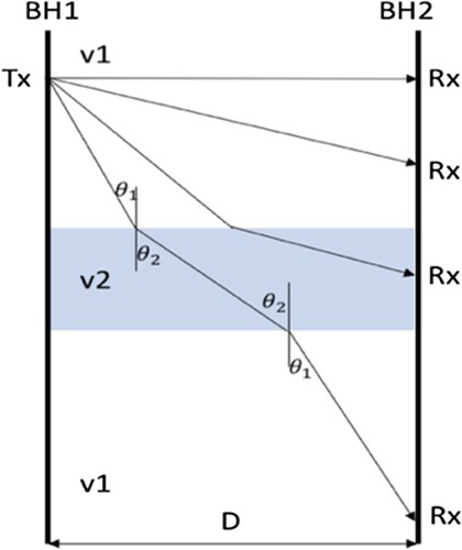
Table 1. Borehole dimension.

Parameter
Depth	20.0 m
Diameter (Inner)	100.0 mm
Casing type	Plastic case (PVC)
Water level	8.5 m
Distance between holes	4.5 m
Direction	Vertical (90°)

Figure 2. (a) GPR profile of the ZOP. The black dashed line indicates the calculated velocity and the water content. (b) Modelled structure with assumed parameters. (c) Simulated GPR profile of ZOP mode.

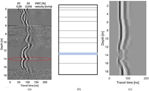
Figure 3. Tomography ray-coverage: (a) Tx: 4 m; (b) Tx: 6 m; (c) Tx: 8 m; (d) Tx: 10 m; (e) Tx: 12 m; (f) Tx: 14 m, and; (g) Tx: 16 m. Colour intensity indicates the apparent velocity.

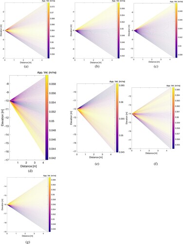
Figure 4. Modelled layers between the boreholes. (a) Antenna is placed at the boundary of the layers (${\epsilon }_{r1}=8$, ${\epsilon }_{r2}=16$). (b) Antenna length is placed in a thin layer (${\epsilon }_{r1}=8,{\epsilon }_{r2}=4$, ${\epsilon }_{r3}=8$). (c) Antenna length is placed in a thin layer (${\epsilon }_{r1}=8,{\epsilon }_{r2}=16$, ${\epsilon }_{r3}=10$). The solid black line indicates a layer boundary.

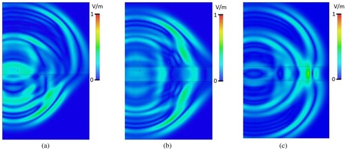
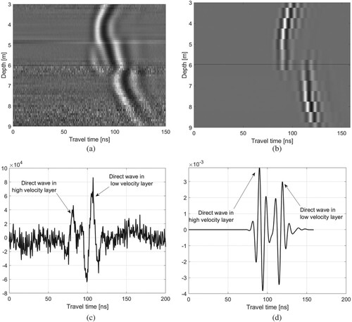
Figure 5. GPR profiles of the simulated data. (a) Low-contrast layer. (b) High-contrast layer. The solid black line indicates the boundaries of the thin layer.

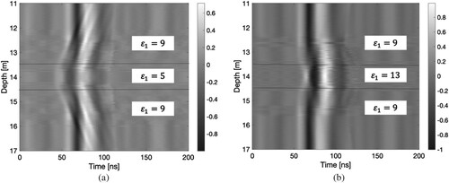
Figure 6. Amplitude profiles of measured data: (a) Tx: 4 m; (b) Tx: 6 m; (c) Tx: 8 m; (d) Tx: 10 m; (e) Tx: 12 m; (f) Tx: 14 m, and; (g) Tx: 16 m.

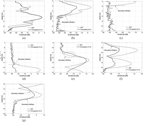
Figure 7. GPR profiles of the fixed transmitter. The solid black line indicates the simulated travel time of the direct waves. The black dashed line indicates the boundary between the layers. (a) Tx = 4 m. (b) Tx = 12 m. (c) Tx = 14 m.

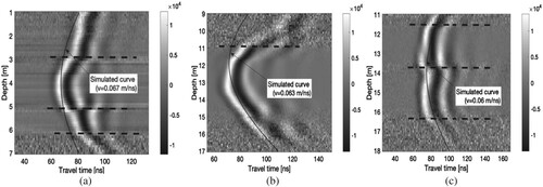
Figure 8. (a) Measured GPR profile. (b) Simulated GPR profile. (c) Measured signal. (d) Simulated signal. The solid black line indicates the selected ray trace.