Figures & data
Figure 1. Area covered by global magnetic data showing a geologic map of structural zones Delamerian and Lachlan Orogens with faults and major zone bounding faults within central and western Victoria (data source: Geoscience Australia and modified in ArcMap after VandenBerg et al. Citation2000). Faults around the northern segment of the Heathcote Fault Zone were modified after Edward et al. Citation2001. The insert Q is where further analysis is performed using aeromagnetic data. Location of profile BB′ across the Newer Volcanic province where the edges of the basaltic extrusives rocks are represented by light grey. The location of previously interpreted seismic lines (1, 2 and 3) and cross-sections of Euler depths (AA′ and BB′) are shown.
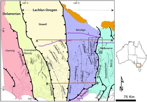
Figure 2. Structural architecture along cross-section AA′ which covers the Stawell, Bendigo and Melbourne Zones. Modified from previous interpretations of seismic lines 1, 2 and 3 covered during 2006 seismic, shows major lithologic units and faults across these structural zones (Cayley et al. Citation2011; Korsch et al. Citation2002).
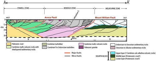
Figure 3. The flowchart illustrates the stages involved in applying our method. The pathway in obtaining optimised clusters is shorter where there are geological or geophysical constraints.
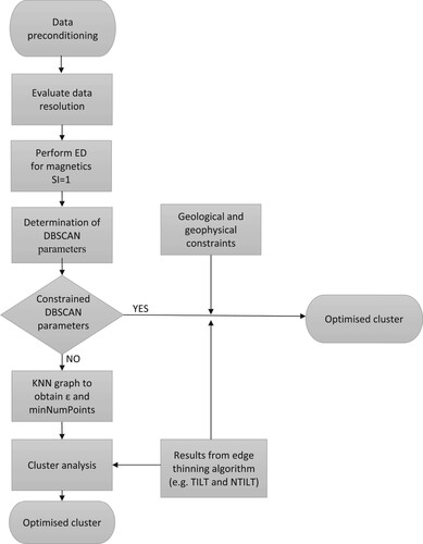
Figure 4. The wavelength components of a 4 × 4° grid of the Reduced to Pole of (a) Earth Magnetic Anomaly Grid (EMAG2; Maus et al. Citation2009) and (b) high-resolution aeromagnetic data (HRAM; Geoscience Australia, 2016). (c) Power spectrum plot of (a) and (b) shows three major spectral zones with a strong correlation of both data at long to medium wavelength zones (see Zone A and B).
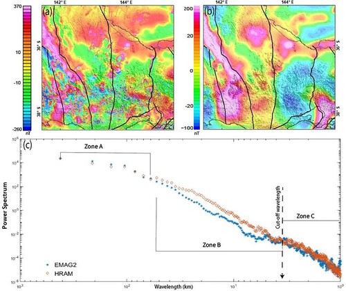
Figure 5. (a) Principle and optimisation of parameters used for DBSCAN required to generate clusters. The K-NN graph shows the number of nearest neighbourhood points (NN) across geologically constrained epsilon (ε) is sorted from farthest away from the ε in Group A to closest in Group D. Cross-section of raw Euler depth results from EMAG2 along profile AA′ (b) and BB′ (c) provides no structural /lithologic information. Location of the profiles is shown in Figure .
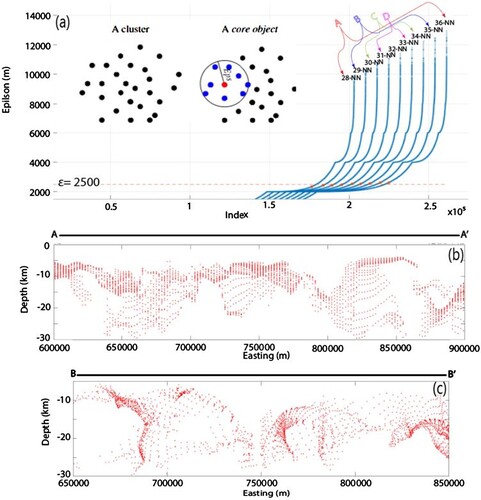
Figure 6. Unconstrained parameters used for clustering depth results obtained from HRAM. (a) The K-NN graph shows a noticeable jump over an ε of 800 in a window between 12 and 19-the minimum number of points derived from the raw cross-section of Euler depth solutions shown in (b).
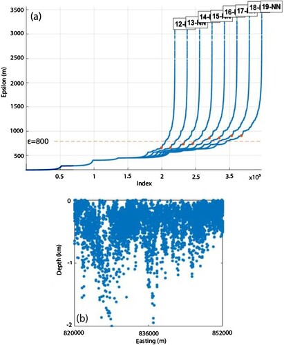
Figure 7. Plan view of Euler depth solutions derived from EMAG2 on the topographic map and their correlation along major zone bounding faults. (a) Euler depth solutions from SI = 0 and their interpretation in (b). (c) Euler depth solutions from SI = 1 and its corresponding interpretation in (d). Euler depth solutions in both cases appear to cluster more along the hangingwall of the major zone-bounding faults.
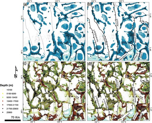
Figure 8. Correlation of Euler depth solutions generated from RTP of the aeromagnetic data using SI = 1. (a) shows the data with no annotation, while (b) shows the locations of the major faults in the vicinity of the Heathcote Fault Zone (locations in Figure ). Concentric clusters of relatively deep depth values correlate with mappable late Devonian granites G1, G2, G3 and G4 (see Edwards et al. Citation2001). Profile C-C′ shows where the cross-section of the Euler depth from the aeromagnetic data is located (Figure ).
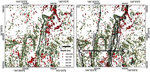
Figure 9. DBSCAN clustering of cross-section AA′ using ε = 2500 m and individual K-NN values and grouped according to their mirror distance from the inflexion point on the K-NN graph in Figure a. (a) End-member cluster assemblages farthest and (D) is the closest to the inflexion point or optimal cluster assemblages. The distinct cluster assemblages are identified by their colours. The n on each cluster assemblage for individual K-NN values indicates the number of clusters or cluster labels. All depth solutions are projected to GDA94/MGA 54.
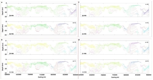
Figure 10. Euler depth solutions across profile B-B′ clustered according to optimised parameters derived from profile A-A′. Also, note the short path to achieve geologically relevant clusters along B-B′ (see Figure ).
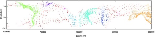
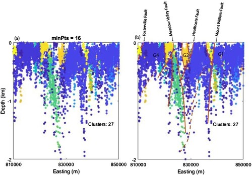
Figure 11. DBSCAN clustering of Euler depth solutions derived from HRAM across profile C-C′, the Heathcote Fault Zone, for each cluster assemblage using ε = 800 m and K-NN values, from 12 to 19, as shown in Figure . Clustering shown in (a) and (g) are end-member cluster assemblages. Cluste assemblages (b) and (h) are regarded as outliers. (d) and (e) are regarded as the optimised cluster assemblages. All depth solutions are projected to GDA94/MGA 54.
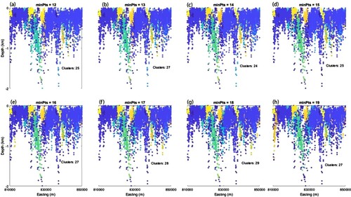
Figure 12. Optimised clustered Euler depth solutions of the cross-section along profile A-A′. Cluster boundaries strongly correlate with the locations of the major zone-bounding faults at depth. The first-order cluster boundaries are in red and, other cluster boundaries, in black.
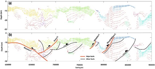
Figure 13. Crustal architecture beneath the Newer Volcanic Province derived from interpreted clustered Euler depth solutions along the B-B′ traverse. (a)Uninterpreted cluster assemblage (b) Interpreted cluster assemblages.
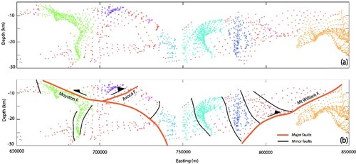
Figure 14. Geologic interpretation of optimised clustering of Euler depth solutions generated from higher resolution airborne magnetic data along profile C-C′ (Figure ). Depth clusters denoted as G1, G2 and G4 are located beneath concentric clusters in plan view (see Figure ) associated with exposed granitic rocks.