ParkinsoNET: Estimation of UPDRS Score Using Hubness-Aware Feedforward Neural Networks

Figures & data

Figure 1. (a) The nearest neighbor relationship is asymmetric. Some instances never appear as the first nearest neighbor of other instances, although there are some instances that appear frequently as the first nearest neighbor of other instances. (b) Example used to illustrate error correction.

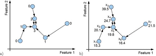
Figure 2. The distribution of in the case of motor UPDRS scores of the telemonitoring dataset for (a) low-error instances, (b) high-error instances, and (c) both histograms in the same plot. Similar observations can be made for the multiple sound recording dataset and total UPDRS scores of the telemonitoring dataset as well. Note that some of the high-error instances appear as nearest neighbors of many other instances, i.e., there are bad hubs in the data. Remarkably, the distribution of high-error instances is shifted to the right compared with the distribution of low-error instances. This indicates that there are more high-error hubs than low-error hubs.

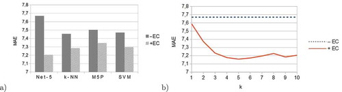
Table 1. Mean absolute error averaged over 10 × 10 folds with (+EC) and without error correction (–EC). The MAE-value is underlined if the difference is statistically significant.

	Motor	Total	Multi	Change motor	Change total
Model	+EC	−EC	+EC	−EC	+EC	−EC	+EC	—EC	+EC	–EC
Net-5	7.206	7.669	9.477	10.080	13.944	14.139	3.150	3.445	3.830	4.117
Net-10	7.232	7.687	9.504	10.056	13.968	14.548	3.148	3.469	3.827	4.127
Net-20	7.276	7.822	9.594	10.065	14.104	14.505	3.136	3.440	3.824	4.109
Net-5,5	7.220	7.558	9.451	10.035	13.764	14.114	3.103	3.473	3.716	4.022
Net-10,10	7.239	7.572	9.476	10.025	13.797	14.145	3.104	3.451	3.718	4.004
Net-20,20	7.266	7.589	9.452	10.014	13.852	14.260	3.106	3.434	3.712	4.013

Figure 3. (a) Performance (MAE) of various models when predicting the motor UPDRS score with (EC) and without (EC) error correction. (b) Performance of Net-5 with error correction (EC) using various -values, and without error correction (EC).