DAG Scheduling in Heterogeneous Computing and Grid Environments Using Variable Neighborhood Search Algorithm

Figures & data

Figure 1. (a) Solution representation. (b) Solution for the problem of 13 tasks and 3 computing nodes. (c) Mapping of tasks with computing nodes for the solution given in (b).

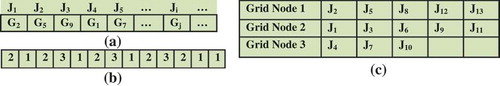
Figure 2. An example DAG(Topcuoglu, Hariri, and Wu 2002).

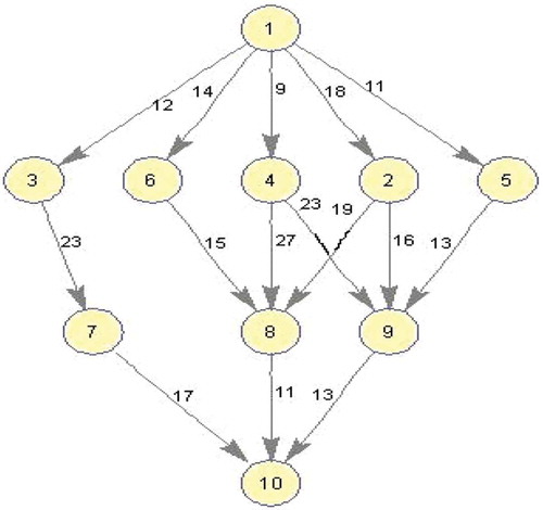
Table 1. Computation cost matrix for random DAG.

Task id	P1	P2	P3
1	14	16	9
2	13	19	18
3	11	13	19
4	13	8	17
5	12	13	10
6	13	16	9
7	7	15	11
8	5	11	14
9	18	12	20
10	21	7	16

Table 2. Upward rank of the tasks.

Task id	Upward rank
1	108.00000
2	77.00000
3	80.00000
4	80.00000
5	69.00000
6	63.33333
7	42.66667
8	35.66667
9	44.33333
10	14.66667

Table 3. Execution order of tasks.

Order of task id
1
4
3
2
5
6
9
7
8
10

Figure 3. Explanation of different neighborhood structures: (a) Initial solution, (b) Weightedmakespan–InsertionMove, (c)Makespan-InsertionMove, (d) BestInsertionMove, (e) SwapMove, (f) InsertionMove, (g) InsertionMove, (h) InsertionMove, and (i) InsertionMove.

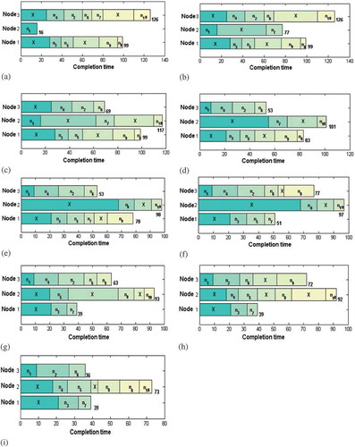
Figure 4. A schedule for the example DAG using the HEFT algorithm.

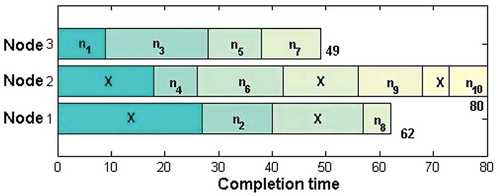
Figure 5. Performance results on random graphs. (a) Average Makespan with respect to DAG size. (b) Average Makespan with respect to CCR.

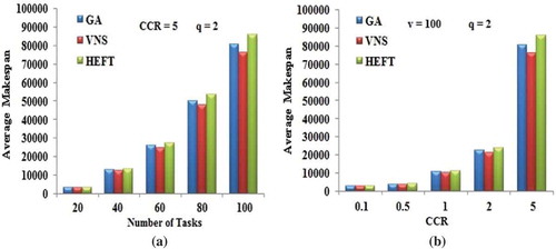
Figure 6. Gaussian Elimination DAG with size 5.

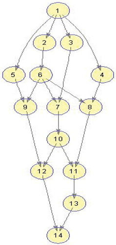
Figure 7. Performance results on Gaussian elimination DAG. (a) Average Makespan with respect to CCR. (b) Average Makespan with respect to number of computing nodes.

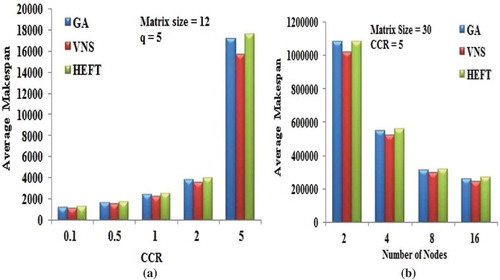
Figure 8. Average Makespan with respect to the matrix size of Gaussian elimination DAG.

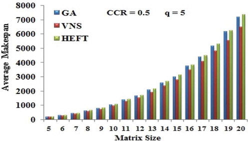
Figure 9. Four input data point FFT DAG.

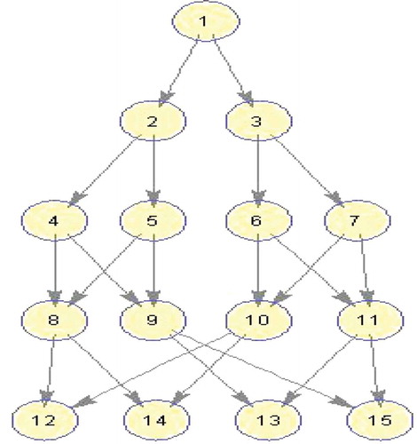
Figure 10. (a) and (b) Average Makespan with respect to the Input data points of FFT DAG.

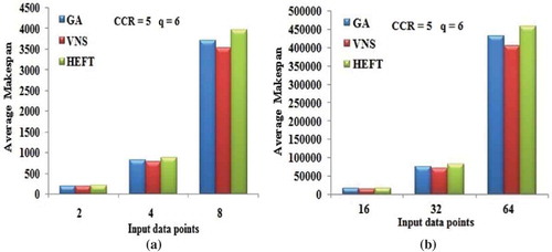
Figure 11. Performance results on FFT DAG. (a) Average Makespan with respect to CCR. (b) Average Makespan with respect to number of computing nodes.

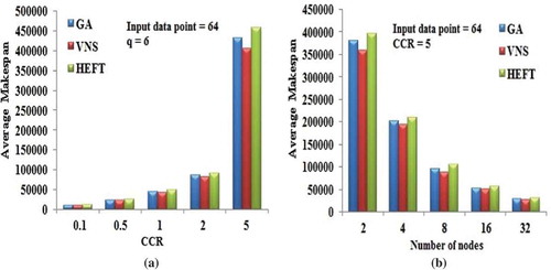
Figure 12. Molecular Dynamics DAG (Topcuoglu, Hariri, and Wu 2002).

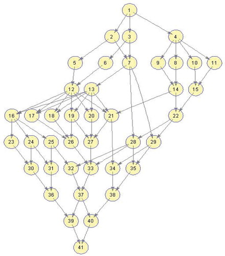
Figure 13. Performance results on Molecular Dynamics DAG. (a) Average Makespan with respect to CCR. (b) Average Makespan with respect to number of computing nodes.

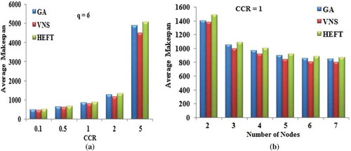
Figure 14. The convergence trace for the Gaussian elimination DAG.

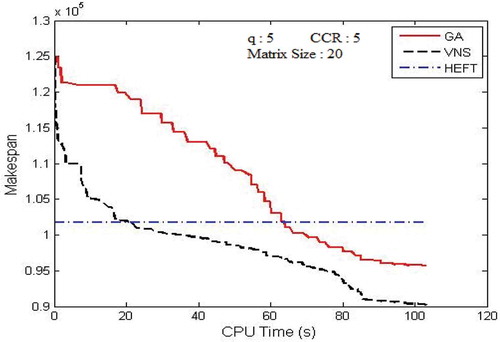
Figure 15. The convergence trace for the fast Fourier transform DAG.

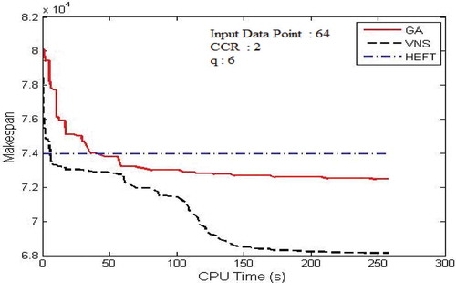
Figure 16. The convergence trace for the molecular dynamics application DAG.

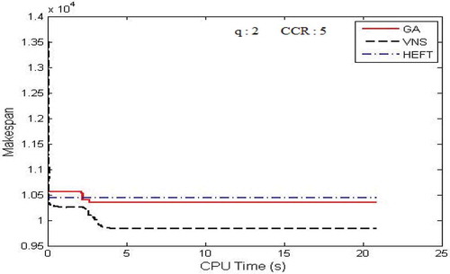
Table 4. Percentage improvement for random graphs with number of tasks.

Number of Tasks with CCR = 5 and q = 2
20			40			60			80			100
VNS		HTPHVNS	VNS		HTPHVNS	VNS		HTPHVNS	VNS		HTPHVNS	VNS		HTPHVNS
Over HEFT	Over GA	Over VNS	Over HEFT	Over GA	Over VNS	Over HEFT	Over GA	Over VNS	Over HEFT	Over GA	Over VNS	Over HEFT	Over GA	OverVNS
6.68	5.74	3.20	7.44	4.68	4.11	9.35	4.79	3.82	10.29	4.18	4.20	10.94	5.20	4.32

Table 5. Percentage improvement for random graphs with different CCRs.

CCR with v = 100 and q = 2
0.1			0.5			1			2			5
.VNS		HTPHVNS	VNS		HTPHVNS	VNS		HTPHVNS	VNS		HTPHVNS	VNS		HTPHVNS
Over HEFT	Over GA	Over VNS	Over HEFT	Over GA	Over VNS	Over HEFT	Over GA	Over VNS	Over HEFT	Over GA	Over VNS	Over HEFT	Over GA	Over VNS
7.66	5.10	4.29	7.97	6.88	4.17	8.80	6.36	4.03	10.76	6.24	4.6	10.94	5.20	4.72

Table 6. Percentage improvement for Gaussian elimination DAG with different CCRs.

CCR with matrix size = 12 and q = 5
0.1			0.5			1			2			5
VNS		HTPHVNS	VNS		HTPHVNS	VNS		HTPHVNS	VNS		HTPHVNS	VNS		HTPHVNS
Over HEFT	Over GA	Over VNS	Over HEFT	Over GA	Over VNS	Over HEFT	Over GA	Over VNS	Over HEFT	Over GA	Over VNS	Over HEFT	Over GA	Over VNS
9.69	4.05	4.03	10.53	7.17	3.9	11.92	7.29	4.23	11.29	6.47	4.12	10.91	8.79	4.6

Table 7. Percentage improvement for various matrix sizes of Gaussian elimination DAG.

	CCR = 0.5 and q = 5
	VNS		HTPHVNS
Matrix size	Over HEFT	Over GA	Over VNS
5	10.18	2.02	4.30
6	10.45	2.27	4.07
7	10.39	6.17	4.12
8	10.16	4.94	3.90
9	9.99	7.11	4.32
10	9.49	6.61	4.15
11	10.12	8.70	4.07
12	10.53	7.17	3.49
13	10.66	8.57	3.72
14	10.79	7.72	4.13
15	10.99	6.66	4.01
16	9.63	7.68	3.97
17	9.33	6.88	3.89
18	9.33	7.21	4.92
19	11.13	9.89	4.01
20	11.81	9.68	4.67

Table 8. Percentage improvement for Gaussian elimination DAG with the number of nodes.

Number of nodes with matrix size = 30 and CCR = 5
2			4			8			16
VNS		HTPHVNS	VNS		HTPHVNS	VNS		HTPHVNS	VNS		HTPHVNS
Over HEFT	Over GA	Over VNS	Over HEFT	Over GA	Over VNS	Over HEFT	Over GA	Over VNS	Over HEFT	Over GA	Over VNS
5.77	5.49	3.97	7.14	5.09	3.91	7.99	5.14	3.67	9.67	5.28	4.12

Table 9. Percentage improvement for FFT DAG with different CCRs.

CCR with input data point = 64 and q = 6
0.1			0.5			1			2			5
VNS		HTPHVNS	VNS		HTPHVNS	VNS		HTPHVNS	VNS		HTPHVNS	VNS		HTPHVNS
Over HEFT	Over GA	Over VNS	Over HEFT	Over GA	Over VNS	Over HEFT	Over GA	Over VNS	Over HEFT	Over GA	Over VNS	Over HEFT	Over GA	Over VNS
8.35	2.82	3.16	9.43	3.85	3.99	9.68	2.46	4.13	10.50	4.18	3.98	11.42	5.85	4.21

Table 10. Percentage improvement for FFT DAG with number of nodes.

Number of nodes with input data point = 64 and CCR = 5
2			4			8			16			32
VNS		HTPHVNS	VNS		HTPHVNS	VNS		HTPHVNS	VNS		HTPHVNS	VNS		HTPHVNS
Over HEFT	Over GA	Over VNS	Over HEFT	Over GA	Over VNS	Over HEFT	Over GA	Over VNS	Over HEFT	Over GA	Over VNS	Over HEFT	Over GA	Over VNS
9.59	5.53	4.25	7.23	4.02	4.10	15.78	7.49	3.86	12.40	5.50	3.97	14.30	6.89	3.78

Table 11. Percentage improvement for various input data points of FFT DAG.

	CCR = 0.5 and q = 5
	VNS
Input data points	Over HEFT	Over GA	Over VNS
2	7.64	2.86	3.04
4	10.13	3.88	3.80
8	10.67	4.53	4.18
16	12.37	3.36	4.22
32	12.88	4.73	3.97
64	11.42	5.85	4.13

Table 12. Percentage improvement for molecular dynamics DAG with the value of CCR.

CCR with q = 6
0.1			0.5			1			2			5
VNS		HTPHVNS	VNS		HTPHVNS	VNS		HTPHVNS	VNS		HTPHVNS	VNS		HTPHVNS
Over HEFT	Over GA	Over VNS	Over HEFT	Over GA	Over VNS	Over HEFT	Over GA	Over VNS	Over HEFT	Over GA	Over VNS	Over HEFT	Over GA	Over VNS
9.52	4.79	4.09	9.34	4.45	4.13	8.93	5.74	3.97	11.30	8.18	4.31	11.18	7.96	4.87

Table 13. Percentage improvement for molecular dynamics DAG with number of nodes.

	CCR = 1
	VNS		HTPHVNS
Number of nodes	Over HEFT	Over GA	Over VNS
2	7.06	1.39	3.01
3	7.95	4.77	4.12
4	8.19	4.99	4.23
5	8.34	6.48	3.94
6	8.93	5.74	3.79
7	8.53	5.85	3.69

Topcuoglu, H., S. Hariri, and M. Y. Wu. 2002. Performance-effective and low-complexity task scheduling for heterogeneous computing. IEEE Transactions Parallel and Distributed Systems 13 (3):260–74. doi:10.1109/71.993206.

 Web of Science ®Google Scholar