A Comparative Analysis of SVM and IDNN for Identifying Penguin Activities

Figures & data

Figure 1. The automatic classifier consists of two stages: the filter stage and the classification stage. The raw dataset can be used as direct input to the classification stage, or can be input to the filter stage. The filter stage elaborates the raw dataset, thus generating a preprocessed dataset. The preprocessed dataset is then used as input to the classification stage. The output is the classification of the data, in this case as “prey handling” or “swimming”.

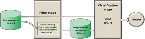
Table 1. The number of neurons that compose an input sequence in each dataset configuration.

Dataset	#Input neurons
Raw (R)	30
Down-sampled (D)	15
Standard deviation (S)	3
Features extracted (F)	22
Normalized Features extracted (FN)	22

Figure 2. The IDNN with the raw sequence input of 30 data points. The hidden layer is composed of five neurons and the output layer is composed of one classification neuron.

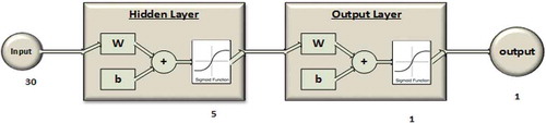
Table 2. The quantity of weights for each dataset configuration combined with the different number of hidden neurons is computed by multiplying the number of input neurons in Table 1 with the number of hidden neurons, each weight is eight bytes. For example, an IDNN with a raw data sequence (30 input neurons) and five hidden neurons needs five lots of 30 weights for the hidden layer.

Dataset	5 hidden neurons	50 hidden neurons	100 hidden neurons
R	150	1500	3000
D	75	750	1500
S	15	150	300
F	110	1100	2200
FN	110	1100	2200

Table 3. Shown here is the memory required for each best-SVM-x and best-IDNN-x configuration as well as their corresponding accuracy. The second column lists the memory required by the SVM for each selected model, and the same applies for the IDNN in the third column. The memory is in kilobytes. The fourth column gives the accuracy provided by the selected models of SVM and the fifth by the selected models of IDNN.

Dataset	SVM memory requirement (kB)	IDNN memory requirement (kB)	SVM accuracy	SVM F1score	IDNN accuracy	IDNN F1score
R	1169	1	81.7%	81.1%	79.2%	79.5%
			(± 0. 003)	(±0.0028)	(± 0. 008)	(± 0. 008)
D	403	0.6	79.8%	80.5%	78.1%	78.5%
			(± 0.005)	(±0.0020)	(± 0.004)	(±0.0064)
S	40	0.11	75.7%	86.2%	76.5%	85.9%
			(± 0.018)	(±0.0000)	(± 0.004)	(±0.0036)
F	214	0.85	84.5%	90.1%	85.2%	90.5%
			(± 0.006)	(±0.0007)	(± 0.005)	(±0.0036)
FN	222	0.8	84.9%	90.4%	84.5%	90.1%
			(± 0.005)	(±0.0005)	(± 0.004)	(±0.0037)

Figure 3. This figure shows the accuracy achieved with the selected model for SVM and IDNN for each configuration of the first stage. The horizontal axis denotes the acronyms referring to each given configuration: Raw (R), Down-sampled (D), Standard deviation (S), Features extracted (F) and Normalized Features extracted (F.N.). The vertical axis displays the accuracy. Light green represents the accuracy of best-IDNN-’x’, and dark green the accuracy of best-SVM-’x’.

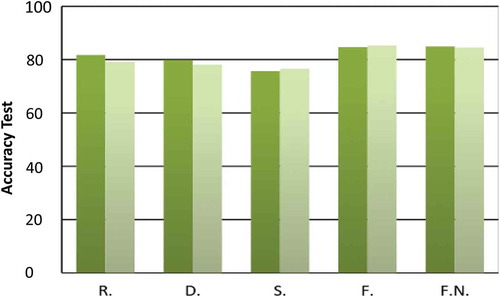
Table 4. The table lists the number of support vectors identified for each selected model of SVM. The first column is the selected model. The second column is the number of support vectors identified for the current model. The third column lists the dimension for each SV.

Selected model for configuration	#support vectors (SV)	Dimension of SV
Best-SVM-R	4991	30
Best-SVM-D	3441	15
Best-SVM-S	1731	3
Best-SVM-F	1248	22
Best-SVM-FN	1292	22

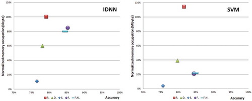
Figure 4. Normalized memory occupation versus accuracy for the different datasets and models. Figure 4a refers to the IDNN model applied to the different datasets, and the memory occupation is normalized assuming 1 to be 1 kB. Figure 4b refers to the SVM model applied to the different datasets, and the memory occupation is normalized assuming 1 be 1 mB.