Figures & data
Table 1. Data represented according to the feature-value format.
Figure 1. Modules of the method developed in this work and their interactions. In particular, the monitor module manages the remaining components, which in turn perform feature selection and multi-objective optimization by a genetic algorithm.
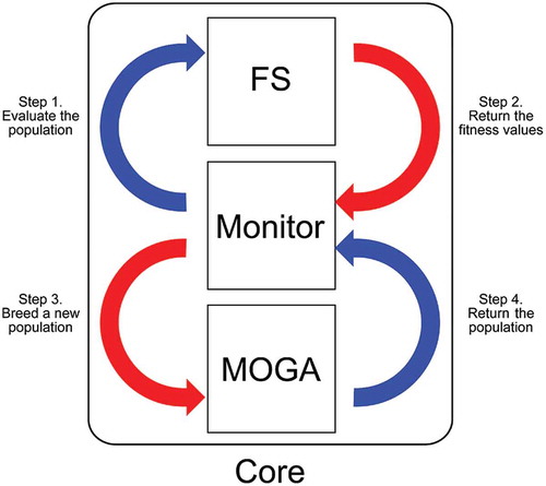
Table 2. Importance measures employed. These measures are associated with distinct categories and can deal with Quantitative (QT) and Qualitative (QL) feature values.
Figure 2. Frequency of related papers per year of publication.
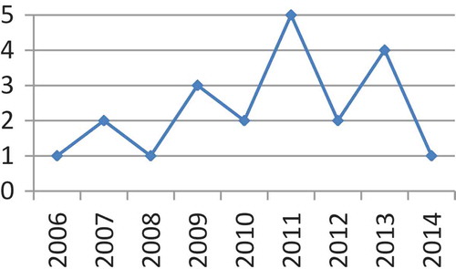
Figure 3. Percentage of related papers using specific numbers of datasets.
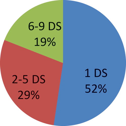
Figure 4. Categories of feature importance measures used in related work.
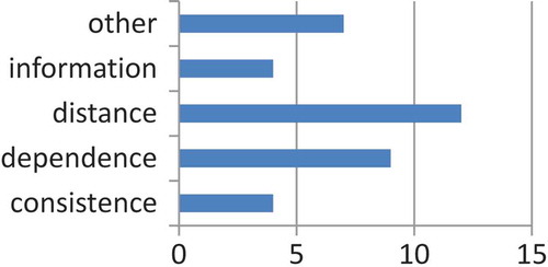
Figure 5. Experimental flow adopted in the evaluation of FS.
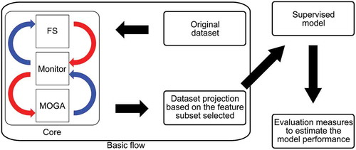
Table 3. Summary of the datasets used in this study: Australian (A), Crx (C), Dermatology (D), German (G), Ionosphere (I), Lung cancer (L), Promoter (P), Sonar (S), Soybean small (Y), Vehicle (V), Wisconsin Breast cancer (B) and Wine (W).!
Figure 6. Comparison procedure based on error rate (axis X) and size of feature subsets (axis Y) (Lee, Monard, and Wu Citation2006).
Table 4. Percentage of Reduction (PR) in the number of features for each dataset. Cells with average PR greater than 50% are highlighted in bold.
Table 5. Performance of J48 and SVM models for each dataset. Cells regarding FS algorithms that obtained PR () greater than 50% are highlighted by an asterisk (*). Cells in italics indicate models with accuracy worse or equal to the Majority Class Error.
Table 6. Performance of NB and NN models for each dataset. Cells regarding FS algorithms that obtained PR () greater than 50% are highlighted by an asterisk (*). Cells in italics indicate models with accuracy worse or equal to the Majority Class Error.
Figure 7. Graphic summary of the predictive performance results. In particular, each bar consists in the area of a polygon in which each axis represents the average accuracy achieved by a specific classifier and FS algorithm.
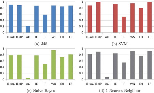
Figure 8. Total number of classifiers built using features selected by the MOGA and SOGA filters for each category related to the trade-off between percentage of reduction in the number of features and classification accuracy.
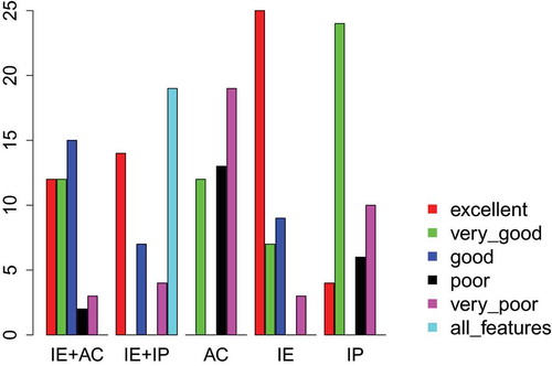
Table 7. Comparison of SVM models built after FS. This comparison involves categorizing the models into six categories regarding the compromise between dimensionality reduction and prediction performance: excellent (▴▴▴), very good (▴▴), good (▴), poor (), very poor (▾) and all features (—).
Figure 9. Graphic comparison of SVM models built after FS with statistical test results.
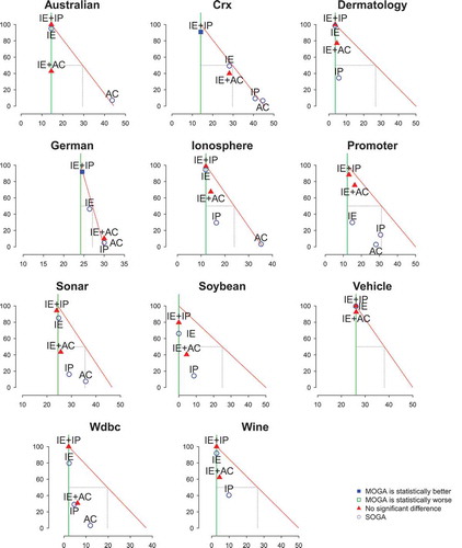
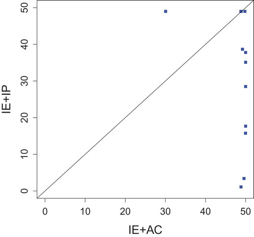
Figure 10. Comparison between MOGA in terms of the number of non- dominated solutions.