Effect of Label Noise on Multi-Class Semantic Segmentation: A Case Study on Bangladesh Marine Region

Figures & data

Figure 1. Statistical representation of label noise (Frenay and Verleysen 2013). NCAR (a) (Noisy completely at random) is an acronym for noisy completely at random. NAR (b) stands for noisy at random. NNAR (c) stands for noisy not at random.

Figure 2. (a) Bangladesh geographical location. (b) High-resolution satellite image of target Region. (c) Targeted marine region.

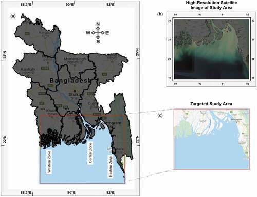
Figure 3. Image labeling and band extraction (a) 12-band satellite image. (b) Labeling with google earth engine. (c) Generating shapefile by QGis Software. (d) Adding shapefile as the 13^th band to the original image.

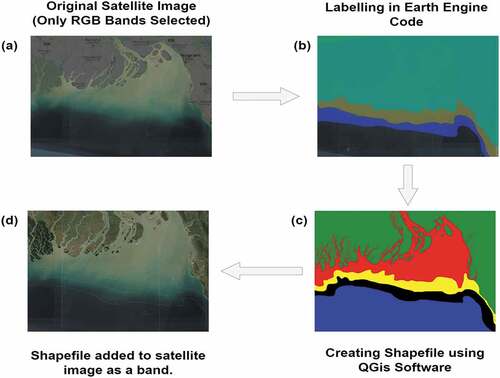
Figure 4. Preparing dataset from the satellite image. (a) 4-band satellite image (4^th band is a label). (b) Stacked layers of an image. (c) The first three layers (bands) are separated as the image. (d) 4^th band is separated as a mask.

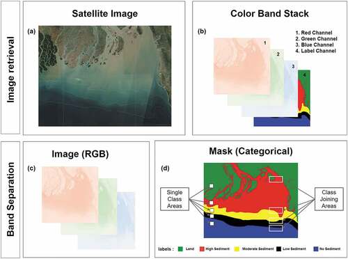
Figure 5. Modified U-Net architecture used in this study.

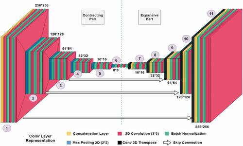
Figure 6. Dice coefficient during training and validation over 30 epochs.

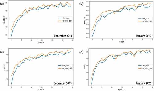
Figure 7. Loss during training and validation over 30 epochs.

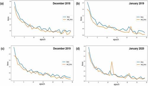
Table 1. Performance measurement for four-year dataset.

	Dice coefficient (%)	Validation dice coefficient (%)	Loss	Validation loss	Validation loss (%)	Validation pixel accuracy (%)
December 2018	85.51	85.42	0.695	0.667	74.88	73.34
January 2019	86.72	86.76	0.627	0.614	77.47	77.07
December 2019	86.86	87.81	0.628	0.600	77.00	78.97
January 2020	85.76	86.22	0.672	0.661	75.25	75.83

Figure 8. Prediction on regions with two class.

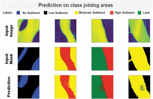
Figure 9. Prediction on regions with one class.

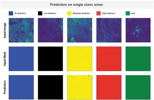
Figure 10. Example of complete random label noise in a range from 1% to 25%.

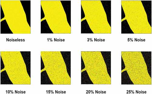
Table 2. Dice coefficient, pixel accuracy, and loss for complete random label noise.

Noise (%)	Dice coefficient (%)	Validation dice coefficient (%)	Loss	Validation loss	Pixel accuracy (%)	Validation pixel accuracy (%)
1%	87.51	87.42	0.595	0.607	78.88	78.34
3%	85.02	86.15	0.734	0.703	74.99	76.44
5%	83.94	85.33	0.796	0.752	72.16	75.11
10%	82.85	83.94	0.874	0.843	71.48	73.35
15%	81.14	81.70	0.954	0.952	69.07	69.40
20%	79.18	79.76	1.03	1.02	65.11	65.85
25%	78.65	79.20	1.07	1.05	64.11	65.21

Figure 11. Class-join prediction under complete random label noise.

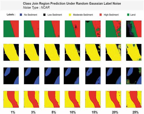
Figure 12. Single-class region prediction under random Gaussian label noise.

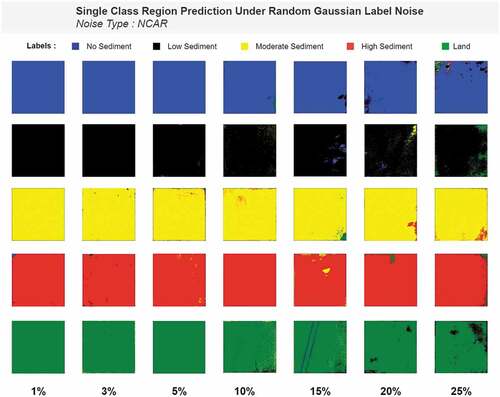
Figure 13. Example of rotational label noise (10^◦ to 40^◦) with nearest fill mode.

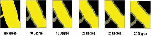
Figure 14. Class-join region prediction under rotational label noise.

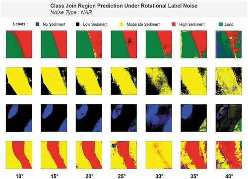
Figure 15. Single class prediction under rotational noise ranging from 10^◦ to 30^◦.

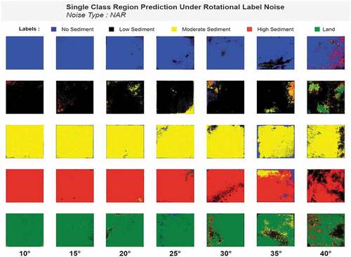
Table 3. Dice coefficient, pixel accuracy, and loss for rotational label noise.

Rotation	Dice coefficient (%)	Validation dice coefficient (%)	Loss	Validation loss	Pixel accuracy (%)	Validation pixel accuracy (%)
10◦	88.46	87.54	0.562	0.610	80.78	78.21
15◦	87.53	87.65	0.616	0.613	79.09	79.01
20◦	85.43	86.76	0.705	0.649	74.49	77.14
25◦	80.78	81.14	0.717	0.726	72.28	71.84
30◦	71.23	73.26	0.958	0.918	67.35	68.16

Figure 16. Example of horizontal and vertical flip label noise.

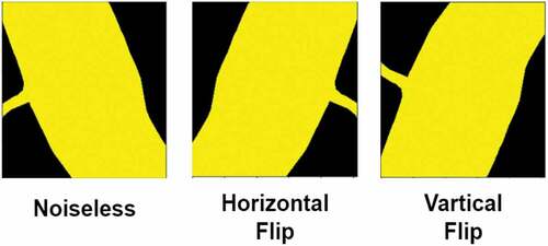
Figure 17. Class-join region prediction under horizontal and vertical flip label noise.

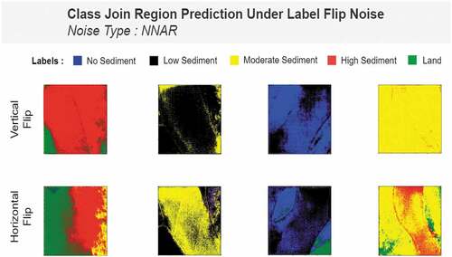
Figure 18. Single-class region prediction under horizontal and vertical flip label noise.

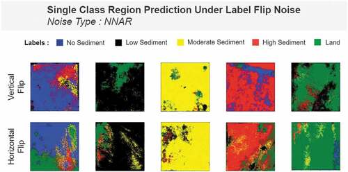
Table 4. Dice coefficient, pixel accuracy, and loss for label flip noise.

Flip	Dice coefficient (%)	Validation dice coefficient (%)	Loss	Validation loss	Pixel accuracy (%)	Validation pixel accuracy (%)
Horizontal	65.94	63.83	1.365	1.647	61.50	63.23
Vertical	67.53	64.65	1.416	1.513	63.09	62.01

Frenay, B., and M. Verleysen. 2013. Classification in the presence of label noise: A survey. IEEE Transactions on Neural Networks and Learning Systems (IEEE) 25 (5):845–69. doi:10.1109/TNNLS.2013.2292894.

 Web of Science ®Google Scholar