Figures & data
Figure 1. Sample frames of lidar data. The top and bottom rows show depth (range) and intensity data, respectively.
Figure 2. Examples of noisy segmented silhouettes from flash lidar data.
Figure 3. Pipeline for gait recognition using the joint correction criterion of GlidarPoly. EquationEquation (4)(4)
(4) describes how depth data are combined with the output of a 2D skeleton detector (skeleton joints in the 2D image frame of reference) to create the 3D location of the joints in the real-world frame of reference.
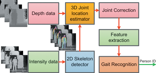
Figure 4. Pipeline for outlier removal. Inputs to “3D Joint location estimator” remain the same as in .
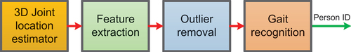
Figure 5. Top row: sample frames with correctly detected skeletons, bottom row: frames with faulty skeletons.
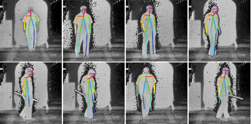
Figure 6. The skeleton model that we use in this work. Left: index of each joint in the skeleton model. Right: skeleton model in a sample frame.
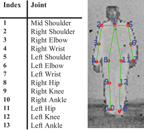
Figure 7. Illustration of length-based feature vectors. Left: description of each feature (L and R refer to the left and right joints, respectively). Right: illustration of the features.
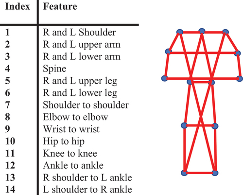
Figure 8. Illustration of vector-based feature vectors. Left: description of each feature (L and R refer to the left and right joints, respectively). Right: illustration of the features.
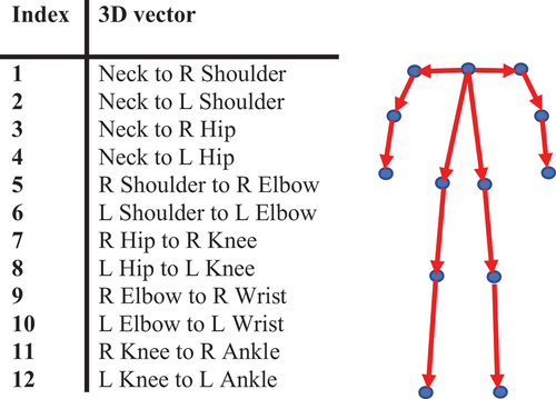
Figure 9. Effect of joint location sequence filtering. From top: sample joint location sequences before (first row) and after (second row) joint location sequence filtering (each joint location sequence corresponds with one coordinate () of the location of one joint through time). Notice the abundance of missing values in the first row, which are shown as missing sections of the plotted signal, that have been recovered through the joint correction (figures in the second row). The last two rows show samples of faulty and missing skeleton joints before (third row) and after (bottom row) joint location sequence filtering.
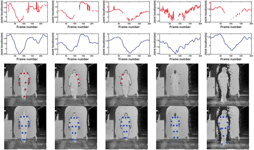
Figure 10. Failure examples of the joint location correction filtering. Sample frames of skeleton joints, before (top) and after (bottom) the joint location correction.
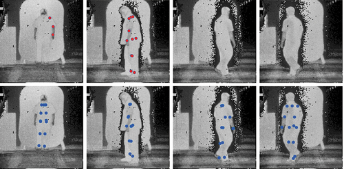
Figure 11. Two examples of the ankle to ankle distance sequence of flash lidar data after joint correction. While the graph on the left presents a clear periodic pattern, the sequence on the right lacks such a pattern.
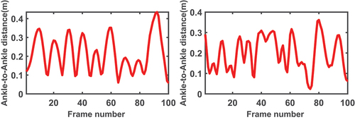
Figure 12. Illustration of two types of waIking paths: walking forward and backward (dashed line) and diamond walking (solid line).
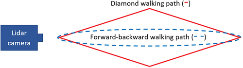
Figure 13. Sample frames of diamond walking that captures a range of different poses.
Table 1. Correct identification scores for the proposed features (**) and the other methods. LB and VB stand for the length-based and vector-based feature vectors, respectively. Results are shown for the original (without joint correction) and after applying GlidarPoly. We also included the results with the proposed features after outlier removal.
Table 2. Correct identification scores with statistics of features computed over gait cycle. LB and VB stand for the length-based and vector-based feature vectors, respectively. The 3-statistic case refers to computing only mean, maximum, and standard deviation of each feature over every gait cycle. The 6-statistic scenario adds median, lower and upper quartile to the initial three statistics.
Table 3. Correct identification scores for each class of subject for the single-shot scenario of vector-based features. The minimum and the next-to-lowest accuracy and F-score are underlined.
Figure 14. T-SNE visualization of the length-based feature before (left) and after (right) applying joint correction. There is a high level of inter-class intersection before joint correction (left) that is mostly resolved after correcting joint location, creating clusters that are more distinctive (right).
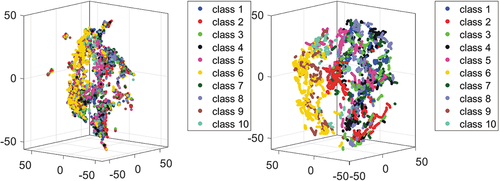
Figure 15. T-SNE visualization of the vector-based feature before (left) and after (right) applying the joint correction. Before joint correction, high inter-class intersection and intra-class separation is observed (left). Joint correction transforms features into well-separated clusters (right).
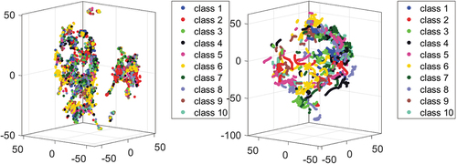
Figure 16. Comparison of classification accuracy for vector-based features based on the number of missing joints in the original skeletons, before and after applying GlidarPoly for joint correction. The samples with no missing joints also include noisy samples. All cases show improvement after applying the joint location correction.
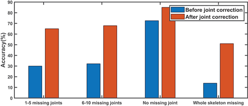
Table 4. Correct identification scores for each class of subject for the statistics of vector-based features over the gait cycle. The minimum and the next-to-lowest accuracy and F-score are underlined.
Figure 17. Average classification accuracy for different sizes of training sample sets given multiple numbers of test examples for the single-shot (left), and statistics over the gait cycle (right) scenarios. Both plots are acquired for vector-based features.
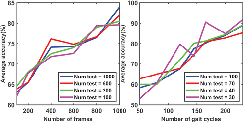
Table 5. Single-shot identification: Rank-1 identification accuracy for the proposed features, several RGB-based (features that are extracted from RGB images), and depth-based (features that are extracted using depth data, e.g. skeleton-based features) features for IAS-Lab RGBD-ID “TestingA” (different outfits) and “TestingB” (different rooms, various illuminations) sets. With (Rao et al. Citation2021), we only report the best results that was achieved by Reverse Reconstruction method. With our features, we only show the best results that was achieved by NN (Nearest Neighbors) and SVM (Support Vector Machine) for the Length-based and Vector-based features, respectively.
Table 6. Single-shot identification: Rank-1 identification accuracy for the proposed features on IAS-Lab RGBD-ID “TestingA” (different outfits) and “TestingB” (different rooms, various illuminations) before (with added noise and removed joints) and after applying GlidarPoly for correction. We only show the best results that was achieved by NN (Nearest Neighbors) and SVM (Support Vector Machine) for the Length-based and Vector-based features, respectively.
Table 7. Rank-1 identification accuracy using the statistics of the proposed features on IAS-Lab “TestingA” (different outfits) and “TestingB” (different rooms, various illuminations) after joint location correction. We only show the best results on average that was achieved by NN (Nearest Neighbors) and SVM (Support Vector Machine) for the Length-based and Vector-based features, respectively.
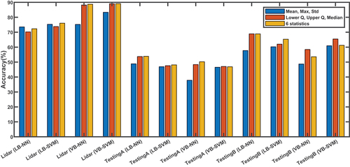
Figure 18. Comparison of the performance of mean, max, standard deviation set, and lower quartile, upper quartile, median set, and the set of all the six statistics to capture the dynamic of the motion after joint location correction. Comparison is performed for lidar and “TestingA” (different outfits) and “TestingB” (different rooms, various illuminations) in IAS-Lab datasets with both types of features and SVM (Support Vector Machine) and NN (Nearest Neighbors) as classifiers. LB and VB stand for length-based and vector-based features, respectively. In the majority of cases, lower quartile, upper quartile, median set outperforms mean, max, standard deviation set.