Physical Domain Reconstruction with Finite Volume Neural Networks

Figures & data

Figure 1. The composition of the modules to represent and learn different parts of an advection-diffusion equation. Red lines indicate gradient flow during training and retrospective inference. Figure from Karlbauer et al. (2022).

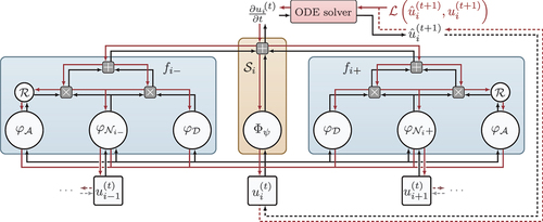
Table 1. Comparison of the training error, test error, and the learnt BC values of all models. For each trial, the average results over 5 repeats are presented. Burgers’ dataset BC $=[1.0,-1.0]$ and Allen–Cahn dataset BC $=[-1.0,1.0]$.

Eqn.	Model	Training Error	Test Error	Learnt BC
Burgers’	DISTANA	$(4.6\pm 3.0)\cdot {10}^{-4}$	$1.69\pm 1.14$	$[0.5460\pm 0.0582,-0.5179\pm 0.0455]$
	PhyDNet	$(2.2\pm 0.5)\cdot {10}^{-5}$	$0.11\pm 0.07$	$[0.3735\pm 0.3259,-0.4068\pm 0.1849]$
	FINN	$(9.6\pm 9.9)\cdot {10}^{-8}$	$5\pm 4\cdot {10}^{-4}$	$[1.0004\pm 0.0002,-1.0004\pm 0.0002]$
Allen–Cahn	DISTANA	$(1.7\pm 2.2)\cdot {10}^{-4}$	$1.50\pm 1.67$	$[-0.5573\pm 0.0372,0.5293\pm 0.0149]$
	PhyDNet	$(6.4\pm 3.1)\cdot {10}^{-6}$	$0.16\pm 0.03$	$[-0.5060\pm 0.0858,0.4438\pm 0.0898]$
	FINN	$(3.4\pm 4.5)\cdot {10}^{-7}$	$1\pm 1\cdot {10}^{-4}$	$[-0.9955\pm 0.0049,0.9994\pm 0.0006]$

Figure 2. Convergence of the boundary conditions and their gradients during training in FINN. The dataset $\mathrm{B}\mathrm{C}=[1.0,-1.0]$ for Burgers’ on the first row. On the second row for Allen–Cahn with $\mathrm{B}\mathrm{C}=[-6.0,6.0].$.

Table 2. Comparison of multi-BC training and prediction errors along with the inferred BC values by the corresponding models. The experiments were repeated 5 times for each trial and the average results are presented. Burgers’ dataset BC $=[3.0,-3.0]$ and Allen–Cahn dataset BC $=[-1.0,1.0]$.

Eqn.	Model	Training error	Test error	Inferred BC
Burgers’	DISTANA	$(3.9\pm 1.2)\cdot {10}^{-5}$	$3.19\pm 0.14$	$[4.4\pm 1.12,-4.0\pm 1.27]$
	PhyDNet	$(1.9\pm 1.0)\cdot {10}^{-4}$	$4.04\pm 0.29$	$[3.6\pm 2.03,-4.4\pm 2.49]$
	FINN	$(1.5\pm 1.3)\cdot {10}^{-7}$	$0.05\pm 0.02$	$[3.1\pm 0.06,-3.1\pm 0.06]$
Allen–Cahn	DISTANA	$(7.6\pm 4.4)\cdot {10}^{-5}$	$0.05\pm 0.02$	$[-1.05\pm 0.189,3.20\pm 2.302]$
	PhyDNet	$(1.2\pm 0.6)\cdot {10}^{-4}$	$0.09\pm 0.07$	$[-1.24\pm 0.524,0.22\pm 0.451]$
	FINN	$(2.6\pm 3.7)\cdot {10}^{-6}$	$(8\pm 8)\cdot {10}^{-6}$	$[-0.99\pm 0.006,0.99\pm 0.005]$

Figure 3. Average prediction errors of 5 multi-BC trained models for Allen–Cahn-Equation. As the BC-range grows larger, the error and the standard deviation (SD) increases. This phenomenon applies to FINN as well (SD range from $4\times {10}^{-6}$ to $1\times {10}^{-3}$). However, due to the scale of the plot, it is not possible to see this shift.

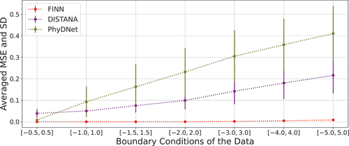
Figure 4. The predictions of the multi-BC trained Allen–Cahn dynamics after inference. First row shows the models’ predictions over space and time. Areas below the red line are the 30 simulation steps that were used for inference and filled with data for visualization. Test error is computed only with the upper area. Second row shows the predictions over $x$ and $u(t=1,x)$, i.e., $u$ in the last simulation step. Data is represented by the red dots and the predictions by the blue line. Best models are used for the plots.

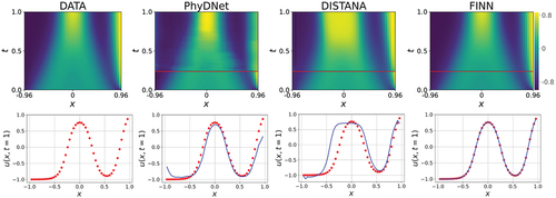
Figure 5. The predictions of the single-BC trained Burgers’ dynamics after inference. First row shows the models’ predictions over space and time. Areas below the red line are the 30 simulation steps that were used for inference and filled with data for visualization. Test error is computed only with the upper area. Second row shows the predictions over $x$ and $u(x,t=2)$, i.e., $u$ in the last simulation step. Data is represented by the red dots and the predictions by the blue line. Best models are used for the plots.

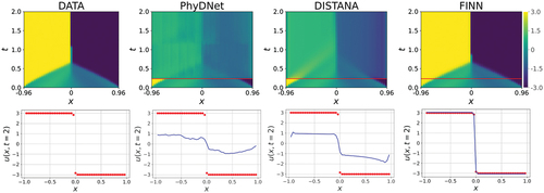
Table 3. Comparison of single-BC training and prediction errors along with the inferred BC values by the corresponding models. The experiments were repeated 5 times for each trial and the average results are presented. Burgers’ dataset BC $=[3.0,-3.0]$ and Allen–Cahn dataset BC $=[-1.0,1.0]$.

Eqn.	Model	Training error	Test error	Inferred BC
Burgers’	DISTANA	$(8.4\pm 1.7)\cdot {10}^{-7}$	$4.14\pm 0.82$	$[-2.5\pm 3.41,+3.0\pm 7.31]$
	PhyDNet	$(1.4\pm 0.9)\cdot {10}^{-4}$	$5.12\pm 0.47$	$[+4.1\pm 3.24,+2.5\pm 8.36]$
	FINN	$(1.7\pm 1.5)\cdot {10}^{-7}$	$0.17\pm 0.16$	$[+3.0\pm 0.01,-3.0\pm 0.01]$
Allen–Cahn	DISTANA	$(1.5\pm 0.4)\cdot {10}^{-5}$	$0.09\pm 0.03$	$[-3.87\pm 3.18,0.12\pm 11.26]$
	PhyDNet	$(4.8\pm 2.2)\cdot {10}^{-5}$	$0.08\pm 0.04$	$[-1.35\pm 1.23,1.92\pm 1.610]$
	FINN	$(2.9\pm 4.2)\cdot {10}^{-6}$	$(1.7\pm 1.4)\cdot {10}^{-5}$	$[-0.99\pm 0.01,0.99\pm 0.006]$

Figure 6. Active tuning algorithm. $R$ corresponds to the retrospective tuning horizon as stated in Otte, Karlbauer, and Butz (2020). The blue column represents the retrospective initial state and the BCs, which are optimized depending on the gradient-signal. The red areas in the middle of the columns are so-called seen areas from which the models receive information and that provide the error signal. The brown areas are called unseen area and models need to reconstruct the equation, i.e., the $u$ values for the entire domain. Black and red arrows represent the model forward and backward passes, respectively. The gradient information (red arrows) is used to infer the BCs.

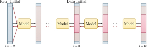
Figure 7. Retrospective state inference. The red lines at $t=0$ show the ground truth, i.e., the initial state of the dataset. The brownish faces indicate the seen area. Best models are used.

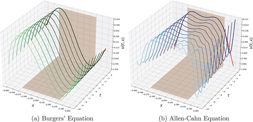
Figure 8. Initial state inference. Figures depict the initial state prediction of the models for $5$ trials. Each light blue line corresponds to one trial. Dataset BC are [1.5, −1.5]. BC-Errors are computed as root mean squared error and are depicted as red lines showing the deviation from the red dots which represent the actual BC values. The plots correspond to the results reported in Table 4.

Table 4. Comparison of seen domain and whole-domain prediction errors along with the inferred BC values by the corresponding models. The experiments were repeated $5$ times for each trial and the average results are presented. Burgers’ dataset BC $=[1.5,-1.5]$ and Allen–Cahn dataset BC $=[-1.0,1.0]$. R = $10$. As 60 data points were used in this experiment (compared to 30 time steps in the previous ones) an error comparison with the other experiments is not possible.

Eqn.	Model	Seen domain error	Whole domain error	Inferred BC
Burgers’	DISTANA	$0.165\pm 0.133$	$0.166\pm 0.136$	$[3.19\pm 0.819,-2.12\pm 0.451]$
	PhyDNet	$0.243\pm 0.056$	$0.715\pm 0.284$	$[0.81\pm 3.415,-0.27\pm 1.314]$
	FINN	$0.006\pm 2\cdot {10}^{-5}$	$0.003\pm 3\cdot {10}^{-5}$	$[1.49\pm 0.008,-1.49\pm 0.003]$
Allen–Cahn	DISTANA	$0.272\pm 0.173$	$0.466\pm 0.422$	$[+1.195\pm 2.76,-1.07\pm 4.02]$
	PhyDNet	$0.517\pm 0.270$	$0.736\pm 0.236$	$[-0.003\pm 0.26,-0.83\pm 1.07]$
	FINN	$(2\pm 0.5)\cdot {10}^{-5}$	$0.013\pm 0.003$	$[-1.038\pm 0.07,+0.67\pm 0.03]$

Figure 9. FINN prediction with noisy data. The red dots show the data and the blue line is the prediction of the model. The area between brown lines indicates the seen area. Best models are used.

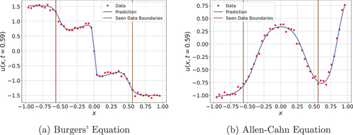
Table 5. Comparison of seen domain and whole-domain prediction errors along with the inferred BC values by the corresponding models inferred on noisy data. The experiments were repeated $5$ times for each trial and the average results are presented. Burgers’ dataset BC $=[1.5,-1.5]$ and Allen–Cahn dataset BC $=[-1.0,1.0]$. R = $10$. As 80 data points were used in this experiment (compared to 30 and 60 time steps in the previous ones) a direct error comparison with the other experiments is not possible.

Eqn.	Model	Seen domain error	Whole domain error	Inferred BC
Burgers’	DISTANA	$0.148\pm 0.080$	$0.160\pm 0.101$	$[4.20\pm 0.919,-3.22\pm 1.480]$
	PhyDNet	$0.259\pm 0.021$	$0.658\pm 0.166$	$[0.45\pm 3.415,-1.83\pm 2.253]$
	FINN	$(9.3\pm 0.3)\cdot {10}^{-3}$	$(5.6\pm 0.2)\cdot {10}^{-3}$	$[1.50\pm 0.016,-1.49\pm 0.010]$
Allen–Cahn	DISTANA	$0.211\pm 0.163$	$0.444\pm 0.428$	$[+0.66\pm 1.414,-0.67\pm 2.621]$
	PhyDNet	$0.603\pm 0.301$	$0.839\pm 0.363$	$[-0.07\pm 0.248,-0.18\pm 0.269]$
	FINN	$(3.94\pm 1.8)\cdot {10}^{-5}$	$0.009\pm 0.011$	$[-0.884\pm 0.44,+0.82\pm 0.141]$

Karlbauer, M., T. Praditia, S. Otte, S. Oladyshkin, W. Nowak, and M. V. Butz. 2022. Composing partial differential equations with physics-aware neural networks. In International Conference on Machine Learning (ICML), Baltimore, USA.

 Google Scholar

Otte, S., M. Karlbauer, and M. V. Butz. 2020. Active tuning. arXiv preprint arXiv:2010.03958.

 Google Scholar