Figures & data
Figure 1. Identification of DE-RBPs and functional enrichment analysis. (A) Volcano plot showing differentially expressed RBPs, DE-RBPs are circled and labeled. (B) Intersection of DEGs and RBPs in renal rejection. (C) Heatmap showing the expression of DE-RBPs in the renal rejection and non-rejection groups. (D, E) Box plots showing expression of DE-RBPs in GSE25902 and GSE48581. (F) GO analysis reveals enrichment of DE-RBPs in biological processes, cellular components, and molecular functions. (G) KEGG pathway analysis of DE-RBPs. (H) Spearman’s correlation analysis showing the correlation of DE-RBPs. *p < .05; ***p < .001; ns: no significance.
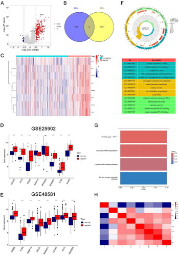
Figure 2. Flowchart of design of this study. RBPs: RNA-binding proteins; KEGG: Kyoto Encyclopedia of Genes and Genomes; GO: Gene Ontology; SVM-RFE: support vector machine recursive feature elimination; GSVA: gene set variation analysis; TCMR: T cell mediated rejection; LASSO: least absolute shrinkage and selection operator; ROC: receiver operating characteristic.

Figure 3. Establishment of renal rejection predictive model. (A) Random Forest Tree. Red represents renal rejection samples, green represents non-rejection samples, and black represents overall samples. (B) Gini importance measure. (C) The SVM-RFE algorithm selects feature RBPs at the optimal point. (D) Boxplot of residuals compares the two models. (E) Cumulative residual distribution plot compares the two models. (F) ROC curves compare the accuracy of the two models. (G) A nomogram model for predicting the risk of renal rejection based on DE-RPBs. (H) Random Forest and SVM-RFE screened hub RBPs take the intersection.
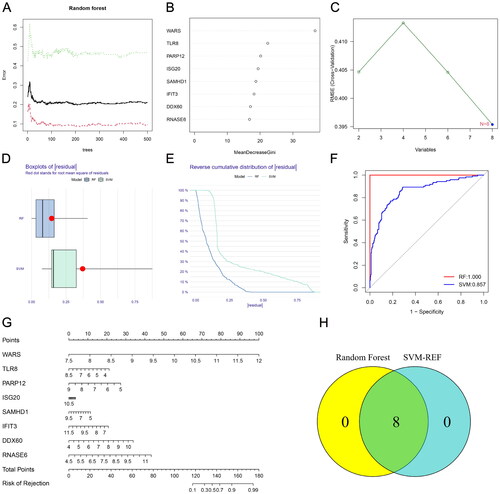
Figure 4. Transplant patients were categorized into two clusters according to hub DE-RBPs using consensus cluster analysis. (A) Consensus matrix of kidney transplant samples when k = 2. (B, C) Relative change in the area under CDF curve and consensus CDF when k = 2–9. (D) Principal component analysis (PCA) showed different expression patterns of the two gene clusters, A and B. (E) K–M survival analysis showed survival differences between the two gene clusters. (F) Box plot showing the expression of hub DE-RBPs between two gene clusters. (G) Heatmap showing the relationship between the expression of hub DE-RBPs and the clinical characteristics of patients in two clusters. ***p < .001.
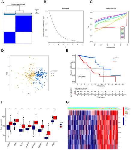
Figure 5. Construction of a predictive signature for long-term survival. (A, B) The 10-fold cross-validation LASSO obtained five candidate RBPs. (C) LASSO coefficients of candidate genes. (D–I) The signature’s K–M survival analysis and time-dependent ROC analysis on the training set, testing set, and whole set. LASSO: least absolute shrinkage and selection operator; K–M: Kaplan–Meier; ROC: receiver operating characteristic curve.
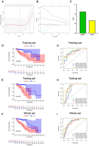
Figure 6. Immune infiltration analysis and risk map of long-term survival predictive signature. (A–C) Risk map of training set, testing set, and overall set. (D) Box plot showing differences in immune cell infiltration between low and high risk groups. (E) Correlation analysis between signature genes and infiltrating immune cells. (F) Sankey diagram showing the relationship between occurrence of rejection, gene clusters, recipient risk, and long-term graft failure. *p < .05; **p < .01; ***p < .001; ns: no significance.
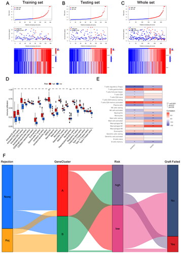
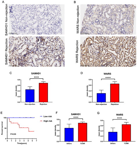
Figure 7. The expression of SAMHD1 and WARS in renal rejection. (A, B) Representative images of immunohistochemical staining of SAMHD1 and WARS in non-rejection and rejection samples. (C, D) Quantitative analysis of immunohistochemical staining of SAMHD1 and WARS in non-rejection and rejection samples. (E) K–M survival analysis in high and low risk groups. (F, G) Quantitative analysis of immunohistochemical staining of SAMHD1 and WARS in TCMR and other samples. ****p < .0001.