Changes in calcareous nannoplankton assemblages around the Eocene-Oligocene climate transition in the Hungarian Palaeogene Basin (Central Paratethys)

Figures & data

Figure 1. Tectonic and geologic setting of the study area. (a) Major structural units of the Pannonian Basin and the surrounding Alpine and Carpathian orogens (modified after Haas 2012). DOB: Dinaridic Ophiolite Belt; MH MU: Mid-Hungarian Mega-unit; TRU: Transdanubian Range Unit; S-U: Sana-Una Unit. (b) Geological sketch map of the Hungarian Palaeogene Basin, showing the location of Cserépváralja-1 (CSV-1) borehole (modified after Nagymarosy 1990)

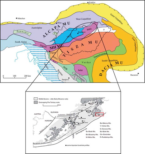
Figure 2. Stratigraphic log of the studied interval of the Cserépváralja-1 drillcore (modified after Ozsvárt et al. 2016), showing the distribution of the identified calcareous nannoplankton species. Black arrows indicate the studied samples

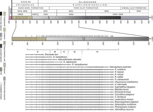
Table 1. The ecological preference and tolerance of the chosen 23 taxa based on published results. We relied on the fundamental works on coccolithophores by Bukry (1974), Perch-Nielsen (1985), Winter and Siesser (1994), Bown (1998) and Thierstein and Young (2004), as well as more recently published comparative studies from Antarctica (Villa et al. 2008), Tanzania (Dunkley Jones et al. 2008), Greece (Maravelis and Zelilidis 2012), Italy (Violanti et al. 2013), Romania (Melinte 2005), Slovakia (Soták 2010) and Hungary (Báldi-Beke 1984; Nagymarosy 1992). The fourth category focuses on the shelf region compared to the open sea (Schneider et al. 2013; Bown and Young 2019). Black-coloured letters indicate information based on published ecological data, green colour shows the confirmed published data in this study, brown colour suggests additional preferences and tolerances for taxa with no published predilection

black published ecological data.

green confirmed in this study.

brown new suggestions based on this study.

Figure 3. Cross-polarised light photomicrographs of selected biostratigraphically and/or palaeoecologically significant calcareous nannofossil taxa. (a) Discoaster barbadiensis Tan. (b) Discoaster saipanensis Bramlette & Riedel. (c) Reticulofenestra reticulata (Gartner & Smith) Roth & Thierstein. (d) Sphenolithus moriformis (Brönnimann & Stradner) Bramlette & Wilcoxon. (e) Reticulofenestra hampdenensis Edwards. (f) Ericsonia formosa (Kamptner) Romein. (g) Clausicoccus subdistichus Prins. (h–i) Zygrhablithus bijugatus (Deflandre in Deflandre & Fert) Deflandre. (j-k) Lanternithus minutus Stradner, (l) Reticulofenestra callida Perch-Nielsen. (m) Helicosphaera euphratis Haq (N) Helicosphaera intermedia Martini. (o) Reticulofenestra bisecta (Hay, Mohler & Wade) Bukry & Percival. (p) Pontosphaera multipora (Kamptner ex Deflandre in Deflandre & Fert Roth. The scale bar is 10 µm

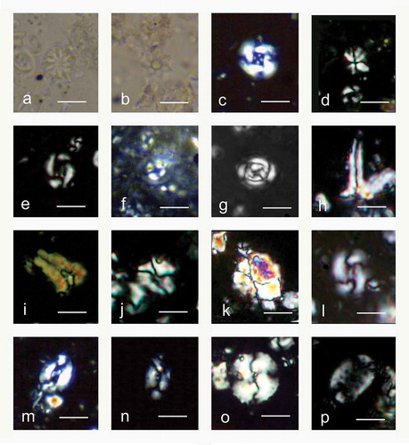
Figure 4. Results of the cluster analysis using Bray–Curtis differences and Ward’s method. (a) Dendrogram of the clustering showing cuts at different heights. (b) Stratigraphic consistency of the grouping achieved at different cutting heights. The x-axis indicates the integer ID value of the sample group and the maximum of each curve indicates the total number of groups in that particular grouping. Decreasing the cutting height from 0.55 progressively increases the number of groups disintegrating Assemblage E in a gradual way

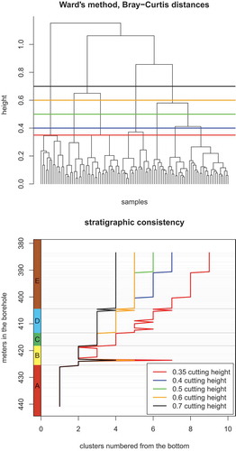
Figure 5. (a) Detrended Correspondence Analysis (DCA) ordination of nannofossil species and samples, where letters indicate the assignment of a sample to one of the assemblages A to E. (a) Distribution of species along axes DCA1 and DCA2. (b) Distribution of species along axes DCA1 and DCA3. (c) Assemblages along axes DCA1 and DCA2. (d) Assemblages along axes DCA1 and DCA3. (e) The relationship between DCA axes and Shannon’s index of diversity (raw). Only DCA2 and DCA3 are associated with sample diversity

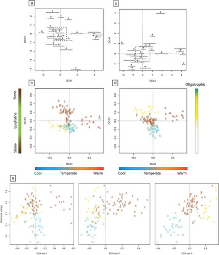
Figure 6. Stratigraphic changes of abundance and diversity of nannoplankton assemblages through Phases A to E. (a) Total abundance of the studied coccolithophores. Average number of specimens in the studied samples. (b) Dominance values in the studied samples. Note that the number of specimens decreases markedly in Phase C, followed by an increase of dominance in Phase D. (c) Species richness in the studied samples. Thick solid line indicates the observed species richness, thin green line indicates standardised richness using classical rarefaction (CR) and dotted lines indicate standardised richness using the SQS method. Note that the richness aspect of diversity remains relatively constant through the section. (d) Shannon’s index of diversity in every sample. Thick solid line denotes raw patterns; thin green line represents values calculated with classical rarefaction

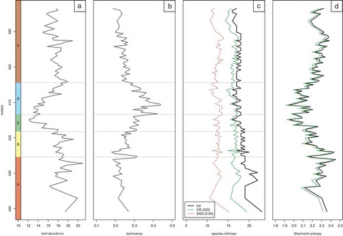
Figure 7. Abundance distribution of paleoecologically significant taxa. (a) Discoaster barbadiensis Tan. (b) Discoaster saipanensis Bramlette & Riedel. (c) Reticulofenestra reticulata (Gartner & Smith) Roth & Thierstein. (d) Sphenolithus moriformis (Brönnimann & Stradner) Bramlette & Wilcoxon. (e) Reticulofenestra hampdenensis Edwards. (f) Ericsonia formosa (Kamptner) Romein. (g) Clausicoccus subdistichus Prins. (h) Zygrhablithus bijugatus (Deflandre in Deflandre & Fert) Deflandre. (i) Lanternithus minutus Stradner, (j) Reticulofenestra callida Perch-Nielsen. (k) Helicosphaera euphratis Haq (l) Helicosphaera intermedia Martini. (m) Reticulofenestra bisecta (Hay, Mohler & Wade) Bukry & Percival. (n) Pontosphaera multipora (Kamptner ex Deflandre in Deflandre & Fert) Roth

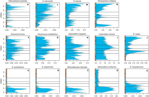
Figure 8. Environmental changes in the section revealed by the distribution of taxa with inferred palaeoecological preferences. (a) Proportion of specimens of species with a preference for cold waters. Note that Phase C and D are characterised by more abundant cold water forms. The grey lines indicate simulation results from 1000 trials, solid line marks the mean, whereas dashed lines mark 1.96 × the standard deviation of the trials. As the randomisation increases the total proportion of cold water forms, the average line of the simulations is shifted away from the real data. Although the confidence intervals are broad, the upper ones in some samples from unit A are lower than the lower confidence intervals of some samples in unit C and D, indicating a significant shift in the proportion of cold water taxa. (b) Proportion of specimens of species with a preference for brackish waters. (c) Proportion of species (blue line) and specimens (black line) with a preference for shelfal habitats

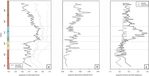
Figure 9. Comparison of the abundance distribution pattern of nannoplankton across the EOT in the CSV-1 core with records from Tanzania (Dunkley Jones et al. 2008) reveals remarkable similarities. A W-shaped pattern is observed as the abundance increases in the late Eocene, followed by a decline then another rise before a pronounced negative trend in the early Oligocene. Comparing the diversity curves between isotope steps 1 and 2, a positive shift is present in both records

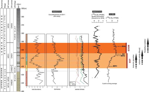
Figure 10. Abundance distribution, dominance and diversity of the 23 significant taxa compared with regional and global δ¹⁸O isotope trends. Highlighted are the 500 ka Eocene-Oligocene transition (EOT, light beige colour), the onset of the Antarctic glaciation and the 400 ka Early Oligocene Glacial Maximum (EOGM, dark orange colour), also showing the beginning of the late Eocene volcanism and the inferred onset of the first isolation event in the Central Paratethys. (Stratigraphy and the oxygen isotope curves are based on Ozsvárt et al. 2016)

Haas J, editor. 2012. Geology of Hungary. Heidelberg: Springer.

 Google Scholar

Nagymarosy A. 1990. Paleogeographical and paleotectonical outlines of some Intracarpathian Paleogene basins. Geol Carpath. 41:259–274.

 Google Scholar

Ozsvárt P, Kocsis L, Nyerges A, Győri O, Pálfy J. 2016. The Eocene-Oligocene climate transition in the Central Paratethys. Palaeogeogr Palaeoclimatol Palaeoecol. 459:471–487.

 Web of Science ®Google Scholar

Bukry D. 1974. Coccoliths as paleosalinity indicators - evidence from Black Sea. AAPG Memoir. 20:353–363.

 Google Scholar

Perch-Nielsen K, editor. 1985. Cenozoic calcareous nannofossils. Cambridge: Cambridge University Press.

 Google Scholar

Winter A, Siesser W. 1994. Coccolithophores. Cambridge: Cambridge University Press.

 Google Scholar

Bown P. 1998. Calcareous nannofossil biostratigraphy. London: Chapman and Hall; Kluwer Academic.

 Google Scholar

Thierstein HR, Young JR. 2004. Coccolithophores: from molecular processes to global impact. Berlin: Springer-Verlag.

 Google Scholar

Villa G, Fioroni C, Pea L, Bohaty S, Persico D. 2008. Middle Eocene–late Oligocene climate variability: calcareous nannofossil response at Kerguelen Plateau, Site 748. Mar Micropaleont. 69:173–192.

 Web of Science ®Google Scholar

Dunkley Jones T, Bown PR, Pearson PN, Wade BS, Coxall HK, Lear CH. 2008. Major shifts in calcareous phytoplankton assemblages through the Eocene-Oligocene transition of Tanzania and their implications for low-latitude primary production. Paleoceanography. 23:PA4204.

 Web of Science ®Google Scholar

Maravelis A, Zelilidis A. 2012. Paleoclimatology and paleoecology across the Eocene/Oligocene boundary, Thrace Basin, Northeast Aegean Sea, Greece. Palaeogeogr Palaeoclimatol Palaeoecol. 365:81–98.

 Web of Science ®Google Scholar

Violanti D, Lozar F, Natalicchio M, Dela Pierre F, Bernardi E, Clari P, Cavagna S. 2013. Stress-tolerant microfossils of a Messinian succession from the Northern Mediterranean basin (Pollenzo section, Piedmont, Northwestern Italy). Boll Soc Paleontol Ital. 52:45–54.

 Web of Science ®Google Scholar

Melinte MC. 2005. Oligocene palaeoenvironmental changes in the Romanian Carpathians, revealed by calcareous nannofossils. Stud Geol Polon. 124:341–352.

 Google Scholar

Soták J. 2010. Paleoenvironmental changes across the Eocene-Oligocene boundary: insights from the Central-Carpathian Paleogene Basin. Geol Carpath. 61:393–418.

 Web of Science ®Google Scholar

Báldi-Beke M. 1984. The nannoplankton of the Transdanubian Palaeogene formations. Geol Hung Ser Palaeont. 43:1–307.

 Google Scholar

Nagymarosy A 1992. Magyarország alsó-oligocén (NP19-24) nannoplanktonjai és ősföldrajzi kapcsolatai [Lower Oligocene (NP19-24) nannoplankton of Hungary and their paleogeographic relations] [Candidate of Science thesis]. Budapest: Hungarian Academy of Sciences.

 Google Scholar

Schneider LJ, Bralower TJ, Kump LR, Patzkowsky ME. 2013. Calcareous nannoplankton ecology and community change across the Paleocene-Eocene Thermal Maximum. Paleobiology. 39:628–647.

 Web of Science ®Google Scholar

Bown P, Young J. 2019. The fossil record of coastal coccolithophores. J Nannoplankton Res. 4:73–80. Special Issue.

 Google Scholar