15,980
Views
302
CrossRef citations to date
0
Altmetric
Articles

On the inner workings of Monte Carlo codes

, &
Pages 1253-1292 | Received 05 Apr 2013, Accepted 18 Jun 2013, Published online: 02 Oct 2013

Figures & data

Figure 1 (Colour online) Ensembles: Shown are the eight ensembles for a single component system. The systems interact through a combined temperature, pressure and chemical potential reservoir. The ensembles on the left are adiabatically insulated from the reservoir, whereas those on the right are in thermal contact with the reservoir. Pistons and porous walls allow for volume and particle exchange. Adiabatic walls are shown cross-hatched, whereas dithermal walls are shown as solid lines. Ensembles on the same height are related by Laplace and inverse Laplace transformations. The pressure stands for the pressure and the tension. Picture taken from Ref. [Citation108].
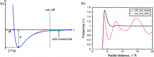
Figure 2 (Colour online) The Lennard-Jones potential has two parameters: the ‘strength’ parameter ϵ and the ‘size’ parameter σ. Energy and force evaluations only take place within the cut-off distance. It is possible to estimate the neglected energy (called the ‘tail’ correction, green area in the picture). For MD, it is customary to use ‘smoothing’ which makes the potential smoothly go to zero at the cut-off (red line). Alternatively, the whole potential can be ‘shifted’ to be zero at the cut-off. The latter leads to continuous forces but remains divergent for higher derivatives. The tail correction calculation assumes that the RDF is approximately unity after the cut-off. The right figure shows that for methane–methane interactions, an arbitrary methane sees an ideal gas of other methane molecule at distances greater than about 12–14 Å for this system. The RDF/tail correction formulation breaks down inside nanoporous materials (here methane in ERI-type zeolites) where the particles are located at adsorption sites in a heterogeneous environment. The RDFs of methane in the fluid and in the pores of ERI are computed at the same density (102 kg/m3).
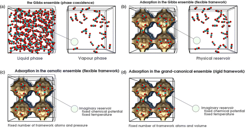
Figure 3 (Colour online) Gibbs, adsorption using Gibbs, the osmotic and the grand canonical ensemble, (a) in the Gibbs ensemble the total volume and the total number of molecules are fixed. The volume move makes one box bigger and the other box smaller which leads to pressure equilibration. The exchange of particles between the boxes leads to equal chemical potential and in both boxes the same temperature is imposed. (b) Adsorption isotherms can be computed in the Gibbs ensemble where the fluid phase is explicitly simulated. (c) The osmotic ensemble replaces the explicit fluid phase by an imaginary reservoir. (d) The grand canonical ensemble also uses the imaginary reservoir but in addition keeps the volume fixed.
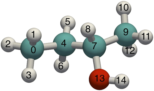
Figure 4 (Colour online) S2butanol: the OPLS definition has 14 bond, 25 bend and 30 torsion potentials. The chiral centre is atom 7.
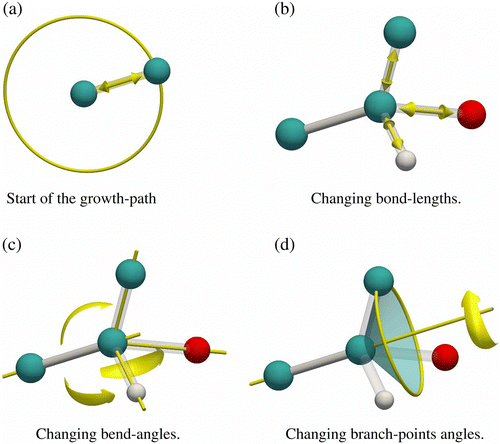
Figure 5 (Colour online) Growing (branched) molecules, (a) bonds are grown by choosing random positions on a sphere; bond lengths (b) and bend angles (c and d) between atoms of a branch are changed by an MC algorithm. The MC moves displace atoms along the bond vectors, or change the bend angle, or rotate the branch atoms around the axis of the bond that was already grown.
Figure 6 (Colour online) NS, (left) first-order transitions are dealt with differently by parallel tempering, Wang–Landau sampling, and NS (right). NS is a top-down approach where a set of random walkers converge downwards in energy at a rate equal to the logarithm of the phase space. Left figure taken from Ref. [Citation256].

Table 1 Energies of a snapshot of 20 CO2 and 10 pentane molecules (TraPPE model) in a  Å box computed with RASPA, TINKER and DLPOLY 4.

Figure 7 (Colour online) Three possible CHA unit cells, (left) primitive cell, (middle) body-centred cell, (right) orthorhombic cell.
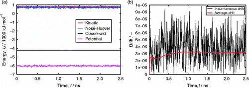
Figure 8 (Colour online) Energy conservation of rigid benzene molecules in MOF-74 at eight molecules per unit cells and 300 K.
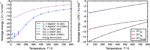
Figure 9 (Colour online) Comparison of average energies (left) using MC, CBMC and MD of methane in MgMOF 74 and CO2 in DMOF at infinite dilution, (right) methane in FAU-type zeolite at N = 96 molecules per unit cell (lines CBMC, points MD). More than cycles were used for the production runs.
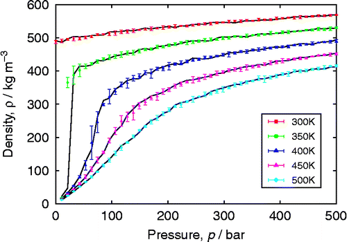
Figure 10 (Colour online) NpT MC (points) versus MD (lines) for fluid properties of propane. MD simulations were run for 500 ps production run; MC used 30,000 initialisation cycles and 50,000 production cycles.
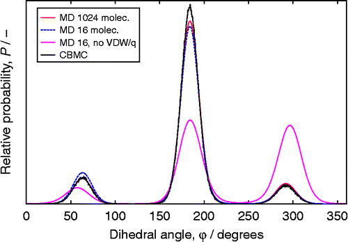
Figure 11 (Colour online) Growing S2butanol, comparison of CBMC and MD at 298 K of the torsional angle of atoms 0-4-7-9 (the four carbons of S2butanol): MD with 1024 and 16 molecules with internal VDW and electrostatics, MD with 16 molecules with no VDW and electrostatic interactions and CBMC.

Table 2 Comparison of CBMC and CFMC for adsorption of CO2 and CH4 in MFI, as a function of fugacity f.
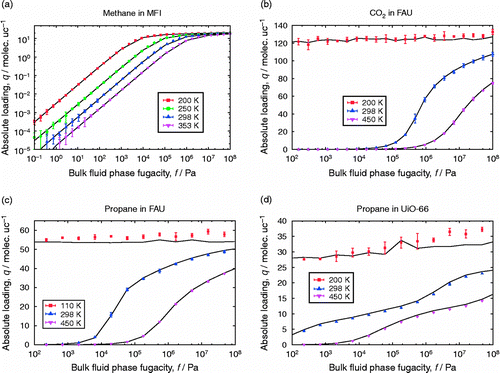
Figure 12 (Colour online) CBMC (lines) versus CFMC (points) for (a) methane in MFI, (b) CO2 in FAU, (c) propane in FAU, (d) propane in UiO-66.CBMC used 150,000 initialisation and 1,500,000 cycles for production; CFMC used 150,000 for initialisation and equilibration and 2,000,000 cycles for production.

Table 3 Gibbs simulations of TraPPE ethane.

Table 4 Gibbs simulations of TraPPE CO2.

Figure 13 (Colour online) CBMC versus CFMC Gibbs comparison of computed coexistence properties, (a) VLE of ethane and CO2 (lines are experimental data taken from NIST), (b) histograms of λ for ethane at 178 K (lines are without biasing; points are with biasing; boxes are the biasing factors).

Table 5 CBMC versus CFMC for an equimolar mixture of CO2/N2 in DMOF at 300 K, with and without the identity switch move.

Supplemental material