Computing properties of the hydrogen dissociation reaction in and away from equilibrium

Figures & data

Figure 1. The inverse thermodynamic correction factor, for a mixture of atomic hydrogen and molecular hydrogen at density and . At this temperature, the degree of dissociation was independent of density within the numerical accuracy of the simulation. The straight lines were fitted in the region in order to find the value in the thermodynamic limit.

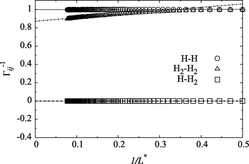
Figure 2. Partial enthalpies determined from fluctuations at (), , as a function of inverse sphere radius for reduced density 0.0003 at . Straight lines were fitted in the region .

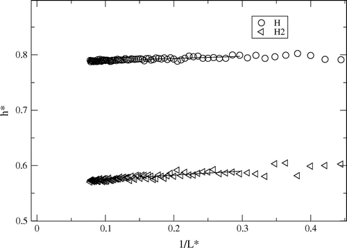
Figure 3. Fluxes of hydrogen molecule, and atom, through the box. The total mass flux, , is constant as no net mass flux is present. The constant a, obtained from the fit, is indicated on the right side of the figure. The temperature gradient was created by velocity swapping (0.17 swaps/fs, with 85% success). See Section 5 for more details on the computational method.

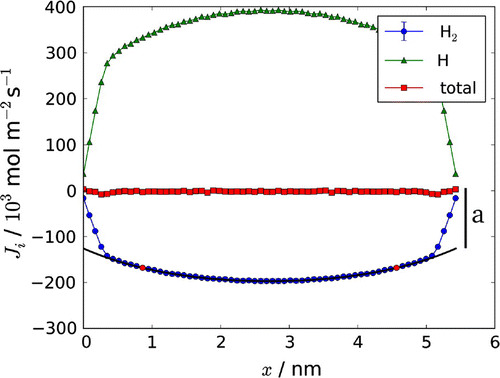
Table 1. Relations between reduced and real units. In this study 51991 K, and  kg.

Reduced variables	Formula
Mass
Distance
Energy
Time
Temperature
Density
Pressure
Velocity	vv

Table 2. The thermal gradient was found from the indicated points (red) in the temperature profile, see Figure . Cases 1a–1d have been performed for the same average temperature, 10,400 K. The success of the thermostat was measured by the number of successful velocity swaps that meet the energy criterion.

Case no.	T(l / 2)		dT/dx	Swap frequency	Success rate
	K	K		fs	%
1a	10.5	-1430	-3.9	0.17	85
1b	10.4	-1070	-2.9	0.13	87
1c	10.3	-940	-2.6	0.10	88
1d	10.4	-750	-2.2	0.08	89
2	15.7	-1210	-3.3	0.10	89

Table 3. The corrected total heat flux, , measurable heat flux, and the corrected mass flux , at (l / 2).

Case
	W m	W m	mol m
1
2

Table 4. Number of H atoms (), mole fraction (), total pressure () and the dissociation constant () for the density, .

	0.07	0.15	0.2	0.25	0.3	0.4
	8	254	477	574	711	761
	496	373	261	213	145	120
	0.984	0.595	0.353	0.270	0.169	0.136
	–	0.276	1.183	1.973	4.088	5.502
	1.138	3.045	4.672	6.347	7.983	11.148

Figure 4. The inverse thermodynamic correction factor in the thermodynamic limit, for the mass densities .

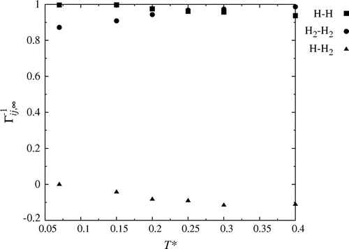
Table 5. Partial enthalpies, at , in the thermodynamic limit. Values are given in reduced units.

0.07	0.34	-0.46
0.15	0.60	0.18
0.2	0.79	0.57
0.25	0.98	0.95
0.3	1.19	1.31
0.4	1.59	2.04

Figure 5. Partial enthalpy in the ensembles; , and . Open symbols corresponds to values for H, while closed symbols represent H.

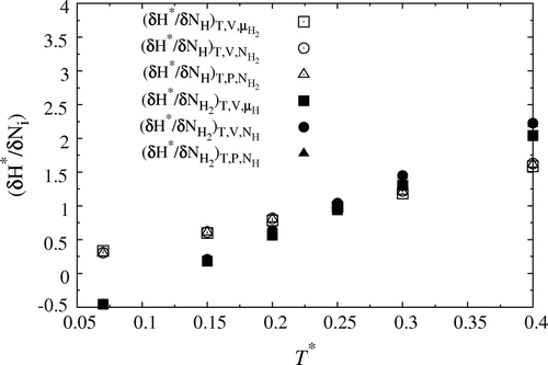
Figure 6. Reaction enthalpy, , as a function of temperature. The points () represent results the simulation, where . The polynomial line represents the fit of the reaction enthalpy to a temperature function. The straight line represents the constant ideal result [11] found by plotting as a function of temperature (1 / T).

Table 6. and as a function of the temperature.

0.15	604	628	1.0
0.2	3208	4126	0.8
0.25	8606	9344	0.9
0.3	16564	24356	0.7
0.4	37932	45778	0.8

Figure 7. The average of six runs of an inverse temperature profile through the box. Error bars are shown. The inverse temperature profile was fitted, according to procedures described in the text, to (Equation (52(52) )). The red markers indicate the start and stop of the fit.

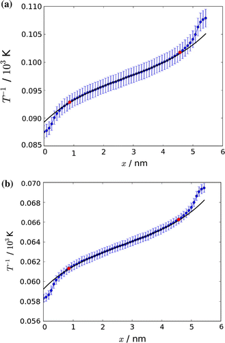
Figure 8. Mole fraction of H and H, , along the simulation box (a), and measurable heat flux, , with the reaction enthalpy carried by the molecule, , along the simulation box (b).

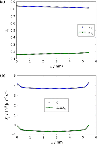
Table 7. Constants from fit to mass flux according to procedures described in the text. Case 1 is the average of Cases 1a–d.

Case			l / d
	mol m s	mol m s	–
1
2

Table 8. Constants obtained from the fit of the inverse temperature profile, as described in the text. Case 1 is an average of Cases 1a–d.

Case
	K	K m	K
1
2

Table 9. Forward rate constant, , penetration depth, d, and mean free path of hydrogen, . Case 1 is an average of case 1a–d

Case		d
	m mol
1			10
2			10

Figure 9. (a) The variation in the net reaction rate, r, and the forward reaction rate, (b), and in the dimensionless chemical driving force through the box. The approximate expression Equation (42(42) ) to the driving force is also shown in Figure (b).

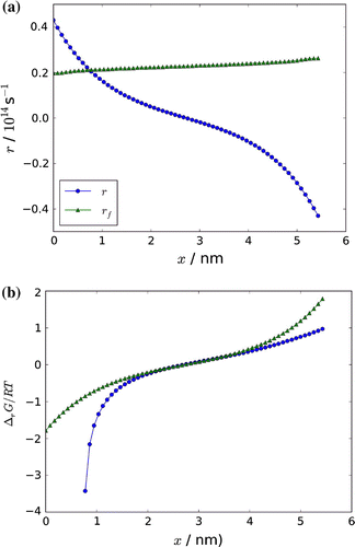
Table 10. Resistivities to transport of heat and mass for various sets of fluxes and forces (see text for definitions).

	m W K	ms mol K	J ms mol K	m s mol K	J ms mol K
1
2

Table 11. Conductivities for transport of heat and mass for various sets of fluxes and forces (see text for definitions).

	W K m	mol K m s	mol K,J ms	W K m	mol K m s
1
2

Table 12. The interdiffusion constant, from simulations () and kinetic theory () in the centre of the gradient (at l / 2) and the binary diffusion coefficient, , according to Butler and Brokaw [34]. All units are in m s.

Case
2

Table 13. Heat of transfer, , and the thermal conductivities in the absence, and presence, (from ), of a chemical reaction. The reaction enthalpy, 424 kJ mol, refer to the average temperature in Case 1.[11]

Case
	kJ mol	W K m	W K m
1
2

Skorpa R , Simon J-M , Bedeaux D , et al . Equilibrium properties of the reaction {H}{H}. Phys. Chem. Chem. Phys. 2013;6:1227–1237.

 Google Scholar

Butler JN , Brokaw RS . Thermal conductivity of gas mixtures in chemical equilibrium. J. Chem. Phys. 1957;26:1636–1643.

 Web of Science ®Google Scholar