Figures & data
Table 1. Comparison of Intel Xeon processor architectures.
Table 2. Naming convention for the STREAM Benchmarks.
Figure 1. (a) Generation over generation Memory Bandwidth per node comparison with STREAM. (b) Memory Bandwidth per Core comparison with STREAM.
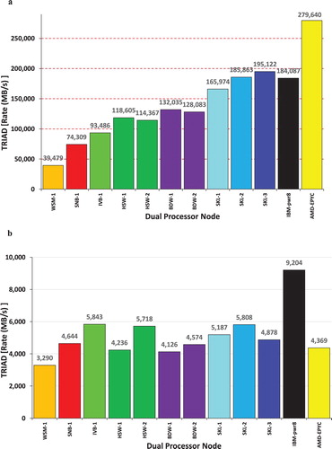
Table 3. Percentage improvement in Time to Solution for DL_POLY Classic and DL_POLY 4 simulations when halving the number of MPI processes per node. Figures are presented as a function of the number of cores.
Figure 2. MPI Benchmark – PingPong performance (MBytes/s) as a function of message size (Bytes) for a number of systems used in the present study.
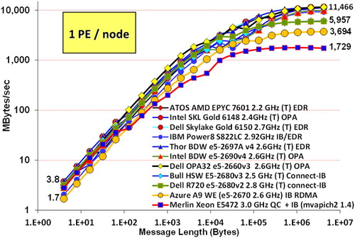
Table 4. Percentage Performance improvement of DL_POLY Classic as a function of compiler option relative to that obtained using –O1.
Table 5. % Performance improvement of DL_POLY 4 as a function of compiler option relative to that obtained using –O1.
Figure 3. IPM Reports for the DL_POLY Classic test cases, Bench4 (i), Bench5 (ii) and Bench7 (iii), showing the fraction of the total simulations time spend in each MPI function.
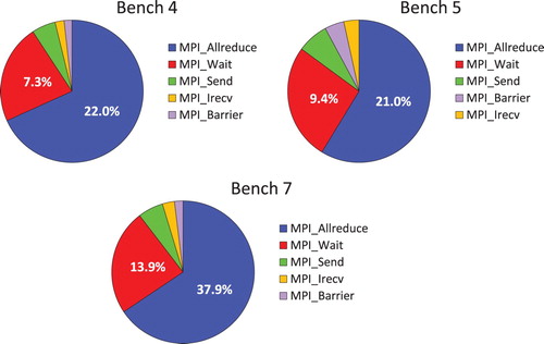
Figure 4. IPM Reports for NaCl (i) and Gramicidin (ii) showing the fraction of the total simulations time spend in each MPI function.
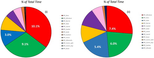
Figure 5. IPM reports for NaCl (i) and Gramicidin (ii) capturing the time spent in each MPI function as a function of Buffer size.
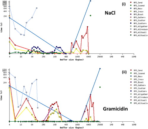
Figure 6. Performance Reports for the DL_POLY 4 NaCl Simulation, (i) Total Wallclock Time Breakdown and (ii) CPU Time Breakdown.
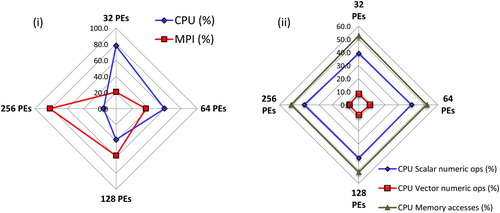
Figure 7. Performance Reports for the DL_POLY 4 Gramicidin Simulation, (i) Total Wallclock Time Breakdown and (ii) CPU Time Breakdown.
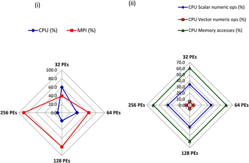
Table 6. HPC and Cluster Systems (CS)a Naming Convention used in analysing the performance of DL_POLY Classic.
Figure 8. Relative performance of the DL_POLY_2 (DL_POLY Classic) NaCl (Bench 4) and Gramicidin (Bench7) simulations on a range of cluster systems using 32 MPI processes (cores) see for the index of Systems.
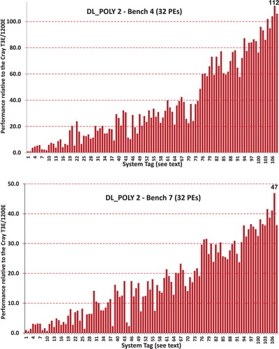
Table 7. Improved Performance of the DL_POLY_2 Bench4 and Bench7 simulations as a function of Intel processor family based on the top SKU systems.
Table 8. Comparison of the SPEC CFP2006 ratings with the measured performance of the DL_POLY Classic Bench4 benchmark.
Table 9. HPC and Cluster Systems Naming Conventiona used in analysing the performance of DL_POLY 3 and DL_POLY 4.
Figure 9. Relative performance of the DL_POLY 3 and DL_POLY 4 NaCl simulation on a range of cluster systems using 32 and 128 MPI processes (see for the index of Systems).
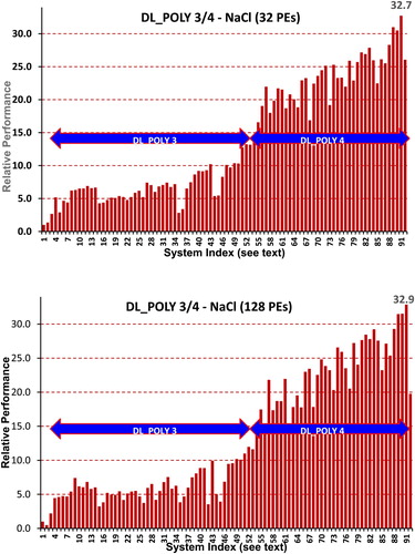
Figure 10. Relative performance of the DL_POLY 3 and DL_POLY 4 Gramicidin simulation on a range of cluster systems using 32 and 128 MPI processes (see for the index of Systems).
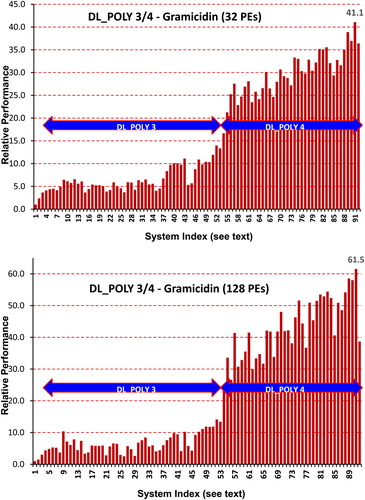
Figure 11. Relative performance of the DL_POLY 4 NaCl and Gramicidin simulations on a range of cluster systems using 128 cores (MPI processes) (see for the index of Systems).
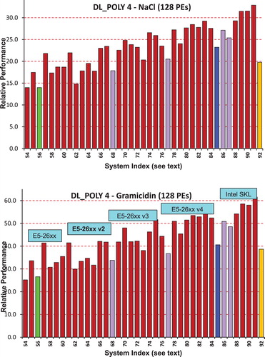
Table 10. Improved Performance of the 32- and 128-core DL_POLY 3/4 NaCl and Gramicidin simulations as a function of Intel processor family based on the optimum SKU systems.
Table 11. Comparison of the SPEC CFP2006 ratings with the measured performance of the DL_POLY 3/ 4 NaCl benchmark.
Figure 12. Performance Comparison as run on the HPC Advisory Council’s Thor Cluster and Intel’s Diamond Cluster for (a) the NaCl simulation, and (b) the Gramicidin simulation.
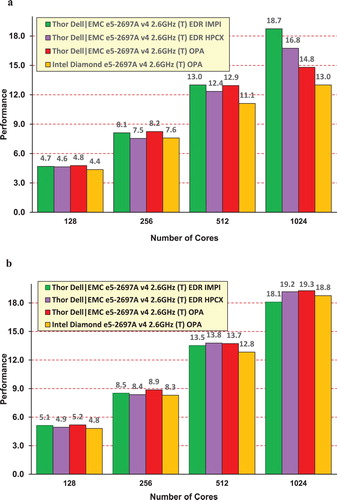
Figure 13. Performance of the DL_POLY 4 NaCl and Gramicidin simulations for a variety of cluster systems (see text)
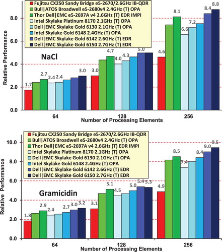
Figure 14. Gramidicin in Water simulation with 99,120 atoms. Strong scalability curves when using one MPI process [left panel] and two MPI processes [right panel].
![Figure 14. Gramidicin in Water simulation with 99,120 atoms. Strong scalability curves when using one MPI process [left panel] and two MPI processes [right panel].](/cms/asset/07638227-b6db-4b87-a767-1c22811a375e/gmos_a_1603380_f0014_oc.jpg)
Figure 15. Optimum performance for two Body Forces on Xeon E2660-v2 (one and two sockets) and Xeon Phi (5110 and 7120), the lower the better. The pale orange area indicates that a tabulated method was used for the potential, while for the green areas, direct evaluation of the potential was used.
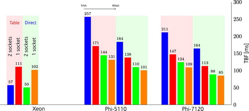
Figure 16. Comparison of runtimes and scaling with different AVX512 flags for Test2 (NaCl) on Intel Xeon Skylake Gold 6142 with Mellanox MT27700 ConnectX-4 interconnect.
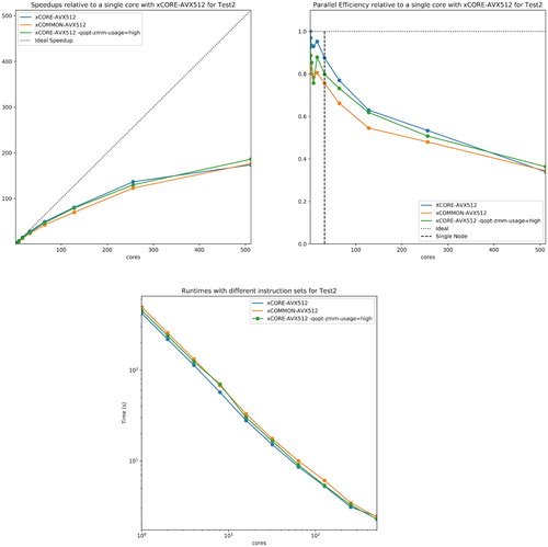
Figure 17. Runtimes and Parallel Efficiency on Xeon Phi KNL 7210 on up to 16 nodes with with Mellanox MT27700 ConnectX-4 interconnect for both Test2 (NaCl) and Test8 (Gramicidin).
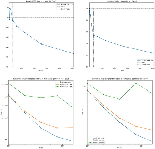
Figure 18. An Intel Advisor Roofline plot for DL_POLY 4 using Test2 on KNL 7210.
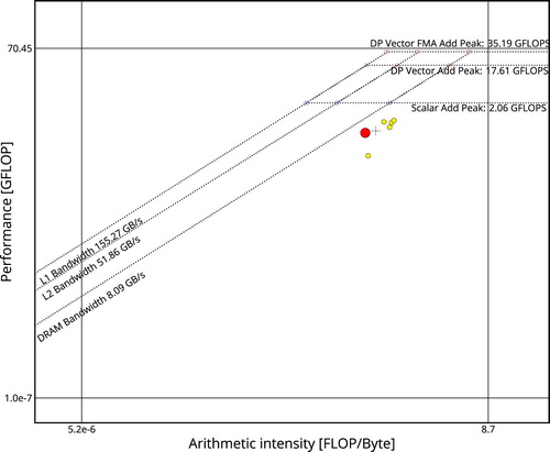
Figure 19. Dual socket Xeon power measurement set up at the Intel Benchmarking Facility.
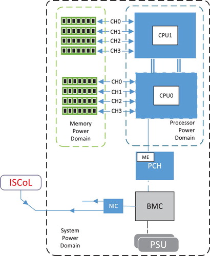
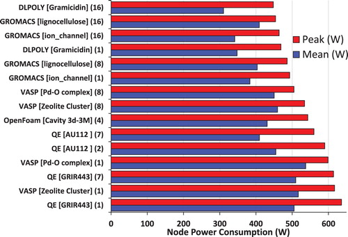
Table 12. Mean and Peak Wattage (W) per node as a function of application and node count.
Figure 20. Mean and Peak power consumptions as a function of application, data set and node count.