Recent advances in the continuous fractional component Monte Carlo methodology

Figures & data

Figure 1. (Colour online) Schematic representation of: (a) test molecule insertions, often resulting in overlaps in dense phases due to the lack of cavities large enough to accommodate test molecules. (b–d) Gradual insertion or removal of a fractional molecule by performing random walks in λ-space. At $\lambda =0$, the fractional molecule does not interact with the other ‘whole’ molecules (ideal gas behaviour) and at $\lambda =1$, the fractional molecule interacts fully with other whole molecules. By performing thermalisation trial moves e.g. translations, rotations, volume moves, etc., the other whole molecules can adapt to the value of λ.

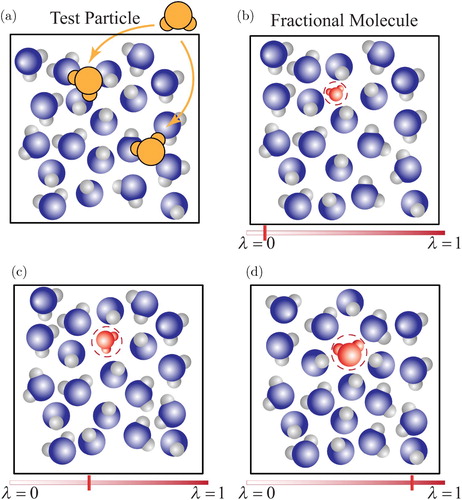
Table 1. A historical overview of the most important methods and developments leading to advancements in staged insertions and free energy calculations in the framework of expanded ensembles.

Year	Author(s)	Method	Application/examples
1920	Born [84]	Using a non-physical pathway for calculating the free energy of ion transfer from the gas to the liquid phase	Free energy calculations in electrolyte solutions
1933	Onsager [80]	Introduction of alchemical (non-physical) parameters to manipulate the intermolecular interaction potential	Free energy calculations in electrolyte solutions
1935	Kirkwood [81]	Introduction of the coupling parameter method and thermodynamic integration	Computation of the chemical potential in a homogeneous fluid
1955	Rosenbluth and Rosenbluth [40]	Self-avoiding random walk for generating polymer conformations with a certain statistical weight	Three-dimensional random walk of chains up to 64 segments
1960	Helfland et al. [90]	Application of the coupling parameter method in scaled particle theory to scale the intermolecular distance between a particle pair	Rigid spheres, square wells, LJ potential
1963	Widom [46]	Widom's test particle insertion method	Lattice-gas model.
1985	Griffiths et al. [55]	Introduction of the gradual insertion and deletion method for computing the chemical potential	Two-dimensional LJ fluid
1988	Harris and Rice [103]	Computation of chemical potentials of chain molecules by discretizing chain conformations	Amphiphilic chains
1990	Siepmann [104]	Direct simulation of flexible chain molecules; combining Widom's test particle insertion method and self-avoiding random walk	Monolayer systems on a lattice
1991	Nezbeda et al. [76]	Combination of gradual test molecule insertion and Widom's test particle insertion method in the NVT ensemble (semi-grand-canonical ensemble) and the grand-canonincal ensemble	Hard-sphere fluid at high densities
1991	Çagin et al. [77]	Introduction of the concept of fractional molecules in grand-canonical MD, evolution of the coupling parameter follows a deterministic approach	Liquid Argon
1991	Kumar et al. [105]	Introducing the chain increment method. Computation of segmental (incremental) chemical potential for chain molecules by appending/removing segments to/from the ghost molecule	Homopolymers in the subcritical and supercritical regime
1992	Kumar [106]	The Hybrid Real Test Particle Method. The test molecule is allowed to move around in the simulation box before deletion.	LJ systems
1992	Lyubartsev et al. [51]	Method of expanded ensembles, free energy differences for a wide temperature range from a single simulation	Hard-core potential (PRM-electrolyte)
1992	Siepmann and Frenkel [65]	Configurational-Bias Monte Carlo (CBMC)	Single chains on a two-dimensional lattice
1992	Frenkel et al. [66]	Extension of the CBCMC to continuously deformable molecules and computation of the chemical potential	Fully flexible chains of 10 to 20 segments
1992	de Pablo et al. [67]	Continuum Configurational Bias (CCB) ghost-chain method. Growing the test molecule segment by segment	Polymeric systems (limited to short chains)
1993	Attard [79]	Computation of the chemical potential using a force-balance Monte Carlo technique	Hard-sphere fluids
1994	Müller et al. [107]	Free energy calculations using thermodynamic integration for excluded volume interactions.	Lattice polymers up to 80 monomers.
1994	Lyubartsev et al. [108]	Combination of the expanded ensemble method and constant temperature MD simulations, stochastic changes of the coupling parameter during the simulation.	LJ and water systems
1994	Wilding et al. [52]	An efficient implementation of the method by Müller et al. Computing the chemical potential by gradually coupling and decoupling a ghost chain molecule in a single simulation [107][107]	Complex polymers, branched or ring structures
1994	Beutler et al. [109]	Introduction of a new functional form for a stable soft-core for efficient free energy calculations for van der Waals and Coulombic interactions	Polar nitrogen atoms and carbon atoms
1994	Kaminsky [93]	Computation of the thermodynamic properties in augmented ensembles, using an intermediate diameter approach	High density LJ fluid
1995	Lo et al. [110]	Introduction of an alternative Hamiltonian and application of a soft core potential in extended grand-canonical MD simulations	Vapor Liquid equilibrium of the LJ system
1995	Escobedo et al. [54]	Introduction of the Expanded Variable Length Chain (EVALENCH) method, single simulation computations using segmental insertions	Polymers applicable to all chain lengths
1996	Escobedo et al. [111]	Improving the efficiency of the EVALENCH method using the Semianalytical Local Mapping (SEAMAP) method	Single simulation of chemical potentials of long chains at high densities
1996	Escobedo et al. [53]	Expanded grand-canonical and Gibbs ensemble simulation of polymers	Hard-core chain fluids and square-well chains
1998	Meirovitc [112]	A tunable method for computing the chemical potential of chain polymers by combining the chain increment method, the scanning method, and a combination of the Rosenbluth technique and the WTPI method	Systems of chaing lengths 30 and 50
1999	Strnada et al. [115]	Computation of the chemical potential in the extended Gibbs ensemble	Binary mixtures of square-well fluid and hard-spheres
2000	Bunker et al. [116]	Parallel excluded volume tempering for polymer chains using a soft core potential	The off-lattice Kremer-Grest model for polymers for lenghts up to 200 monomers
2001	Vlugt et al. [212]	Application of a soft core potential in the grand-canonical ensemble to couple/decouple attractive and excluded volume interactions	Binary LJ systems
2003	Boinepalli et al. [118]	Hybrid MD-MC grand-canonical simulation, the evolution of the coupling parameter is deterministic.	LJ system
2005	Lísal et al. [119]	Expanded-Ensemble Osmotic Molecular Dynamics (EEOMD) method. The changes in the coupling parameter are stochastic using transition probabilities from the grand-canonical ensemble	NaCl in water at ambient conditions
2007	Shi et al. [59]	Continuous Fractional Monte Carlo (CFCMC) using adaptive biasing method in open ensembles (grand-canonical ensemble)	LJ, water, CO-ethanol binary systems
2008	Shi et al. [60]	Extension of the CFCMC method to the Gibbs ensemble	LJ, water, SO2
2011	Pham et al. [120]	Identifying low variance pathways for free energy calculations	Application for a generalized soft-core potential
2011	Rosch et al. [42]	Application of the CFCMC method in the reaction ensemble	Propene methathesis reaction and methyl-tetr-butyl-ether (MTBE) synthesis
2014	Torres-Knoop et al. [121]	CB/CFCMC hybrid method; combination of the CFCMC method with the CBMC method	Single and five-component isomers of hexane in Fe2(BDP)3
2015	Sikora [122]	Combination of the CBCMC and CFCMC methods based on the approach of Torres-Knoop et al. [121]	High density adsorption in metal-organic frameworks
2016	Poursaeidesfahani el al. [123]	Improving the efficiency of the CFCMC method in the Gibbs ensemble by using a single fractional molecule for direct computation of the chemical potential	LJ and water systems
2017	Poursaeidesfahani el al. [61]	Efficient application of the CFCMC method in the reaction ensemble	LJ system and the ammonia synthesis reaction
2017	Yoo et al. [56]	Discrete Fractional Monte Carlo, a modified version of the CFCMC method using discrete staging is used instead of the continuous change of the coupling parameter	C10E4 and water
2018	Mullen et al. [124]	Identity changes between the reactants and reaction products in combination with the CFCMC method (semi-grand trial move)	CO2 absorption in the reactive ionic liquid triethyl(octyl)phosphonium 2-cyanopyrrolide
2018	Rahbari et al. [125]	Computation of partial molar properties by combining the WTPI method and the CFCMC method	Binary LJ color mixture, ternary mixtures of ammonia, nitrogen and hydrogen
2019	Rahbari et al. [126]	An alternative scheme to directly sample the states λ = 1 and λ = 0 leading to an increased accuracy of computed chemical potentials	SPC/E water and TraPPE methanol, LJ systems
2020	Rahbari et al. [127]	Multiple free energy calculations and computation of partial molar properties by combining the CFCMC method and umbrella sampling [128]	Aqueous methanol mixtures and LJ systems

Figure 2. (Colour online) MC trial moves in the CFCMC Gibbs ensemble are used to perform stepwise molecule exchanges between the phases [123]. The coupling parameter λ is used to scale the interactions of the fractional molecule with surrounding molecules. The deletion or insertion of the fractional molecule is staged using the coupling parameter λ. Trial moves to facilitate molecule exchanges are: (a) Random walks in λ-space: attempts to randomly change the value of λ while keeping the positions of all molecules constant. For the cases $\lambda <0$ or $\lambda >1$, the trial move is rejected. (b) Swapping the fractional molecule: the fractional molecule is removed from one simulation box and inserted at a randomly selected position in the other simulation box. The value of λ is not changed in this trial move. (c) Identity changes: an attempt to transform the fractional molecule into a whole molecule, accompanied by changing a randomly selected molecule in the other simulation box into a fractional molecule, while keeping the positions of all molecules fixed. For these trial moves, the acceptance rules are derived in Ref. [123].

Figure 3. (Colour online) Chemical potentials of water (TIP3P [179]) and hydrogen (Marx [180]) from vapour-liquid equilibrium simulations of binary water-hydrogen mixtures in the CFCMC Gibbs ensemble, as a function of pressure, at T=323 K (squares), T=366 K (diamonds), T=423 K (triangles). (a) Chemical potential of water in the liquid phase (closed symbols) and chemical potential of water in the gas phase (open symbols). (b) Chemical potential of hydrogen in the liquid phase (closed symbols) and chemical potential of hydrogen in the gas phase (open symbols). Lines and dashed lines are used as a guide for the eye for the liquid phase and gas phase, respectively. The chemical potentials in this figure are part of the previously published VLE data of water-hydrogen of Ref. [178]. These chemical potentials were not explicitly reported in Ref. [178]. Simulation details on the phase coexistence of the water-hydrogen system are provided in Ref. [178]. Raw data and uncertainties are provided in the Supporting Information. (c) Molecule exchanges between the liquid and the gas phase are performed in a gradual manner using the fractional molecules of water and hydrogen (marked molecules). The snapshot is generated using iRASPA [185].

Figure 4. (Colour online) Trial moves associated with fractional molecules facilitating chemical reactions in the reaction ensemble. The ammonia synthesis reaction ${\mathrm{N}}_2+3{\mathrm{H}}_2\rightleftharpoons 2{\mathrm{N}\mathrm{H}}_3$ is considered as an example to demonstrate the trial moves: (a) Random walks in λ-space: an attempt to change the value of λ while orientations and positions of all molecules are fixed. Here, the coupling parameter is used to scale the interactions of ${\mathrm{N}}_2+3{\mathrm{H}}_2$. (b) Reaction for the fractional molecules; the fractional molecules of reaction products $2{\mathrm{N}\mathrm{H}}_3$ are inserted and the fractional molecules of the reactants ${\mathrm{N}}_2+3{\mathrm{H}}_2$ are removed. The orientations and positions of other molecules are unchanged. (c) Reaction for the whole molecules; randomly selected reaction products ($2{\mathrm{N}\mathrm{H}}_3$) are transformed into fractional molecules and the fractional molecules of the reactants ${\mathrm{N}}_2+3{\mathrm{H}}_2$ are transformed into whole molecules. The acceptance rules for these trail moves are provided in Ref. [61].

Figure 5. (Colour online) (a) Mole fractions of ammonia at chemical equilibrium obtained from Rx/CFC simulations (symbols) and experiments (solid lines) [188] at 573 K (circles), 673 K (upward-pointing triangles), 773 K (squares) and, 873 K (downward-pointing triangles) as a function of pressure. All simulations were started from a random configuration of 120 ${\mathrm{N}}_2$ and 360 ${\mathrm{H}}_2$ molecules and no ammonia molecules. (b) Fugacity coefficients of ammonia at equilibrium obtained from Rx/CFC simulations (symbols) using Equation (13(13) $\prod _{i=1}^R{{\varphi }_i}^{-{\nu }_i}=\left(\frac{p({\lambda }_R=1)}{p({\lambda }_R=0)}\right)\times {\left(Z_{\mathrm{m}}\right)}^{\xi }$(13) ) and the Peng-Robinson EoS (lines) [24] at 573 K (circles), 673 K (upward-pointing triangles), 773 K (squares) and, 873 K (downward-pointing triangles) as a function of pressure. Raw data is taken from Ref. [61].

Figure 6. (Colour online) Reaction enthalpy of the Haber-Bosch process per mole of ${\mathrm{N}}_2$ at pressures between 100 bar and 800 bar, at T=573 K. The reaction enthalpy at P=1 bar is indicated with an arrow on the left hand side of the figure. The contribution of intermolecular interactions to the reaction enthalpy is computed using: Peng-Robinson EoS (upward-pointing triangles); PC-SAFT (downward-poiting triangles); CFCNPT ensemble (circles). No binary interaction parameters were used in the EoS modelling. The data is taken from Ref. [125].

Figure 7. (Colour online) Probability distribution $p(\lambda ,T)$ for pure methanol obtained from CFCNPT simulation at T=298 K and P=1 bar (410 molecules). Equation (17(17) $p\left(\lambda ,P\right)=c\cdot {⟨\delta ({\lambda }^{{}^{\prime }}-\lambda )\exp \left[\text{β}V\left(P^{\star }-P\right)\right]⟩}_{P^{\star }}$(17) ) is used to compute $p(\lambda ,T)$ for temperatures between 329 and 273 K from a single simulation at 298 K. The bold red line indicates the Boltzmann distribution of $p(\lambda ,T=298\mathrm{K})$. The data is taken from Ref. [127].

Born M. Volumen und Hydratationswärme der Ionen. Zeitschrift für Phys Chem. 1920;1:45–48.

 Google Scholar

Onsager L. Theories of concentrated electrolytes. Chem Rev. 1933;13:73–89.

 Google Scholar

Kirkwood JG. Statistical mechanics of fluid mixtures. J Chem Phys. 1935;3(5):300–313.

 Google Scholar

Rosenbluth MN, Rosenbluth AW. Monte Carlo calculation of the average extension of molecular chains. J Chem Phys. 1955;23:356–359.

 Web of Science ®Google Scholar

Helfand E, Reiss H, Frisch HL, et al. Scaled particle theory of fluids. J Chem Phys. 1960;33:1379–1385.

 Web of Science ®Google Scholar

Widom B. Some topics in the theory of fluids. J Chem Phys. 1963;39:2808–2812.

 Web of Science ®Google Scholar

Mon KK, Griffiths RB. Chemical potential by gradual insertion of a particle in Monte Carlo simulation. Phys Rev A. 1985;31:956–959.

 PubMed Web of Science ®Google Scholar

Harris J, Rice SA. A lattice model of a supported monolayer of amphiphile molecules: Monte Carlo simulations. J Chem Phys. 1988;88:1298–1306.

 Web of Science ®Google Scholar

Siepmann JI. A method for the direct calculation of chemical potentials for dense chain systems. Mol Phys. 1990;70:1145–1158.

 Web of Science ®Google Scholar

Nezbeda I, Kolafa J. A new version of the insertion particle method for determining the chemical potential by Monte Carlo simulation. Mol Simul. 1991;5:391–403.

 Web of Science ®Google Scholar

Çagin T, Pettitt BM. Grand molecular dynamics: a method for open systems. Mol Simul. 1991;6:5–26.

 Web of Science ®Google Scholar

Kumar SK, Szleifer I, Panagiotopoulos AZ. Determination of the chemical potentials of polymeric systems from Monte Carlo simulations. Phys Rev Lett. 1991;66:2935–2938.

 PubMed Web of Science ®Google Scholar

Kumar SK. A modified real particle method for the calculation of the chemical potentials of molecular systems. J Chem Phys. 1992;97:3550–3556.

 Web of Science ®Google Scholar

Lyubartsev AP, Martsinovski AA, Shevkunov SV, et al. New approach to Monte Carlo calculation of the free energy: method of expanded ensembles. J Chem Phys. 1992;96:1776–1783.

 Web of Science ®Google Scholar

Siepmann JI, Frenkel D. Configurational bias Monte Carlo: a new sampling scheme for flexible chains. Mol Phys. 1992;75:59–70.

 Web of Science ®Google Scholar

Frenkel D, Mooij GCAM, Smit B. Novel scheme to study structural and thermal properties of continuously deformable molecules. J Phys Condens Matt. 1992;4(12):3053–3076.

 Web of Science ®Google Scholar

de Pablo JJ, Laso M, Suter UW. Estimation of the chemical potential of chain molecules by simulation. J Chem Phys. 1992;96:6157–6162.

 Web of Science ®Google Scholar

Attard P. Simulation of the chemical potential and the cavity free energy of dense hard-sphere fluids. J Chem Phys. 1993;98:2225–2231.

 Web of Science ®Google Scholar

Müller M, Paul W. Measuring the chemical potential of polymer solutions and melts in computer simulations. J Chem Phys. 1994;100:719–724.

 Web of Science ®Google Scholar

Lyubartsev AP, Laaksonen A, Vorontsov-Velyaminov PN. Free energy calculations for Lennard-Jones systems and water using the expanded ensemble method a Monte Carlo and molecular dynamics simulation study. Mol Phys. 1994;82:455–471.

 Web of Science ®Google Scholar

Wilding NB, Müller M. Accurate measurements of the chemical potential of polymeric systems by Monte Carlo simulation. J Chem Phys. 1994;101:4324–4330.

 Web of Science ®Google Scholar

Beutler TC, Mark AE, van Schaik RC, et al. Avoiding singularities and numerical instabilities in free energy calculations based on molecular simulations. Chem Phys Lett. 1994;222:529–539.

 Web of Science ®Google Scholar

Kaminsky RD. Monte Carlo evaluation of ensemble averages involving particle number variations in dense fluid systems. J Chem Phys. 1994;101:4986–4994.

 Web of Science ®Google Scholar

Lo C, Palmer B. Alternative Hamiltonian for molecular dynamics simulations in the grand canonical ensemble. J Chem Phys. 1995;102:925–931.

 Web of Science ®Google Scholar

Escobedo FA, de Pablo JJ. Monte Carlo simulation of the chemical potential of polymers in an expanded ensemble. J Chem Phys. 1995;103:2703–2710.

 Web of Science ®Google Scholar

Escobedo FA, DE Pablo JJ. Chemical potential and dimensions of chain molecules in athermal environments. Mol Phys. 1996;89:1733–1754.

 Web of Science ®Google Scholar

Escobedo FA, de Pablo JJ. Expanded grand canonical and Gibbs ensemble Monte Carlo simulation of polymers. J Chem Phys. 1996;105:4391–4394.

 Web of Science ®Google Scholar

Meirovitch H. Simulation of the chemical potential of polymers. Comput Theor Polym Sci. 1998;8:219–227.

 Google Scholar

Strnada M, Nezbeda I. An extended Gibbs ensemble. Mol Simul. 1999;22:183–198.

 Web of Science ®Google Scholar

Bunker A, Dünweg B. Parallel excluded volume tempering for polymer melts. Phys Rev E. 2000;63:016701.

 Web of Science ®Google Scholar

Vlugt TJH. Measurement of chemical potentials of systems with strong excluded volume interactions by computing the density of states. Mol Phys. 2002;100(17):2763–2771.

 Web of Science ®Google Scholar

Boinepalli S, Attard P. Grand canonical molecular dynamics. J Chem Phys. 2003;119:12769–12775.

 Web of Science ®Google Scholar

Lísal M, Smith WR, Kolafa J. Molecular simulations of aqueous electrolyte solubility: 1. the expanded-ensemble osmotic molecular dynamics method for the solution phase. J Phys Chem B. 2005;109:12956–12965.

 PubMed Web of Science ®Google Scholar

Shi W, Maginn EJ. Continuous fractional component Monte Carlo: an adaptive biasing method for open system atomistic simulations. J Chem Theory Comput. 2007;3:1451–1463.

 PubMed Web of Science ®Google Scholar

Shi W, Maginn EJ. Improvement in molecule exchange efficiency in Gibbs ensemble Monte Carlo: development and implementation of the continuous fractional component move. J Comput Chem. 2008;29:2520–2530.

 PubMed Web of Science ®Google Scholar

Pham TT, Shirts MR. Identifying low variance pathways for free energy calculations of molecular transformations in solution phase. J Chem Phys. 2011;135:034114.

 PubMed Web of Science ®Google Scholar

Rosch TW, Maginn EJ. Reaction ensemble Monte Carlo simulation of complex molecular systems. J Chem Theory Comput. 2011;7:269–279.

 PubMed Web of Science ®Google Scholar

Torres-Knoop A, Balaji SP, Vlugt TJH, et al. A comparison of advanced Monte Carlo methods for open systems: CFCMC vs CBMC. J Chem Theory Comput. 2014;10:942–952.

 PubMed Web of Science ®Google Scholar

Sikora BJ, Coln YJ, Snurr RQ. Continuous fractional component Monte Carlo simulations of high-density adsorption in metal-organic frameworks. Mol Simul. 2015;41:1339–1347.

 Web of Science ®Google Scholar

Poursaeidesfahani A, Torres-Knoop A, Dubbeldam D, et al. Direct free energy calculation in the continuous fractional component Gibbs ensemble. J Chem Theory Comput. 2016;12:1481–1490.

 PubMed Web of Science ®Google Scholar

Poursaeidesfahani A, Hens R, Rahbari A, et al. Efficient application of continuous fractional component Monte Carlo in the reaction ensemble. J Chem Theory Comput. 2017;13:4452–4466.

 PubMed Web of Science ®Google Scholar

Yoo B, Marin-Rimoldi E, Mullen RG, et al. Discrete fractional component Monte Carlo simulation study of dilute nonionic surfactants at the air–water interface. Langmuir. 2017;33:9793–9802.

 PubMed Web of Science ®Google Scholar

Mullen RG, Corcelli SA, Maginn EJ. Reaction ensemble Monte Carlo simulations of CO2 absorption in the reactive ionic liquid triethyl(octyl)phosphonium 2-cyanopyrrolide. J Phys Chem Lett. 2018;9:5213–5218.

 PubMed Web of Science ®Google Scholar

Rahbari A, Hens R, Nikolaidis IK, et al. Computation of partial molar properties using continuous fractional component Monte Carlo. Mol Phys. 2018;116:3331–3344.

 Web of Science ®Google Scholar

Rahbari A, Hens R, Dubbeldam D, et al. Improving the accuracy of computing chemical potentials in CFCMC simulations. Mol Phys. 2019;117:3493–3508.

 Web of Science ®Google Scholar

Rahbari A, Hens R, Moultos OA, et al. Multiple free energy calculations from single state point continuous fractional component Monte Carlo simulation using umbrella sampling. J Chem Theory Comput. 2020;16:1757–1767.

 PubMed Web of Science ®Google Scholar

Torrie GM, Valleau JP. Nonphysical sampling distributions in Monte Carlo free-energy estimation: umbrella sampling. J Comput Phys. 1977;23(2):187–199.

 Web of Science ®Google Scholar

Jorgensen WL, Chandrasekhar J, Madura JD, et al. Comparison of simple potential functions for simulating liquid water. J Chem Phys. 1983;79:926–935.

 Web of Science ®Google Scholar

Marx D, Nielaba P. Path-integral Monte Carlo techniques for rotational motion in two dimensions: quenched, annealed, and no-spin quantum-statistical averages. Phys Rev A. 1992;45:8968–8971.

 PubMed Web of Science ®Google Scholar

Rahbari A, Brenkman J, Hens R, et al. Solubility of water in hydrogen at high pressures: a molecular simulation study. J Chem Eng Data. 2019;64:4103–4115.

 Web of Science ®Google Scholar

Dubbeldam D, Calero S, Vlugt TJH. iRASPA: GPU-accelerated visualization software for materials scientists. Mol Simul. 2018;44:653–676.

 Web of Science ®Google Scholar

Gillespie LJ, Beattie JA. The thermodynamic treatment of chemical equilibria in systems composed of real gases. I. An approximate equation for the mass action function applied to the existing data on the Haber equilibrium. Phys Rev. 1930;36(4):743.

 Google Scholar

Peng DY, Robinson DB. A new two-constant equation of state. Ind Eng Chem Fundam. 1976;15:59–64.

 Web of Science ®Google Scholar