Machine learning and descriptor selection for the computational discovery of metal-organic frameworks

Figures & data

Table 1. A list of metal-organic frameworks with ultra-high Brunauer-Emmett-Teller (BET) surface area and pore volume.

MOF	BET surface area ($m^2{g}^{-1}$)	pore volume ($c{m}^3{g}^{-1}$)	Ref.
NU-110E	7140	4.40	[15]
NU-109E	7010	3.75	[15]
MOF-210	6240	3.6	[16]
NU-100	6140	2.82	[17]
UMCM-2	5200	2.32	[18]
NOTT-116/PCN-68	4660/5110	2.17	[19]
DUT-23-Co	4850	2.03	[20]
MOF-177	4750	1.59	[21]
MOF-205	4460	2.16	[16]
Bio-MOF-100	4300	4.30	[22]
MIL-101c	4230	2.15	[23]
UMCM-1	4160		[24]
Be${}_{12}$(OH)${}_{12}$(BTB)${}_{24}$	4030		[25]
PCN-66	4000	1.36	[26]

Figure 1. (Colour online) Schematic representation of a few MOFs with high gas storage property. As an example, MOF-5 is known for high H${}_2$ storage capacity, and is composed of ZnO (light green), acting as the metal ‘node’ and while benzodicarboxylate serves as the ‘linker’ molecule. Most MOFs have acronymns and they are often named after the institute or place of origin. Reprinted with permission from Acta Crystallographica Section B [30].

Table 2. A list of metal-organic frameworks databases.

Name	Number of MOF structures	Year of development
Univ. of Ottawa	315,615	2016, [48]
CoRE${}^{\mathrm{a}}$	15,000+	2014, Updated on 2019 [44]
h-MOF${}^{\mathrm{b}}$	137,000+	2013 [45]
CSD-integrated toolbox${}^{\mathrm{c}}$	99,075	2020 [49]
ToBaCCo${}^{\mathrm{d}}$	13,512	2017 [50–52]
In silico surface	8815	2015 [53]
In silico deliverable	2816	2015 [54]
Zr-MOFs	204	2014 [55]
Mail-order	112	2013 [56]

${}^{\mathrm{a}}$ CoRE is acronym for Computation-Ready, Experimental,

${}^{\mathrm{b}}$h-MOFs stands for hypothetical MOFs,

${}^{\mathrm{c}}$CSD-integrated toolbox is a dynamic database builder in the Cambridge Crystallographic Data Centre (CCDC) software which serves as a classification system to filter out MOFs based on chemical and physical criteria. The database builder extracts candidates from the larger Cambridge Structure database (CSD) which contains 99075 MOF structures, and

${}^{\mathrm{d}}$ToBaCCo stands for Topologically-Based Crystal Constructor.

Figure 2. (Colour online) A typical machine learning workflow applied to discovery of MOFs. The orange-shaded or the inner region covers the three step process of building an ML model for material discovery (provided the features and training set are available) with the following steps: model selection, model training, and validation. The outer region, coloured in light red, covers the descriptor selection, dataset creation, and model testing parts of the process. This type of inner and outer region representation of the workflow helps us to understand the purpose of the inner region, which is to perfect the model given the dataset and descriptor via traversing these sub-processes: model selection, optimisation, and tuning. The outer region is more focused on handling the dataset and also its best representation in the form of descriptors.

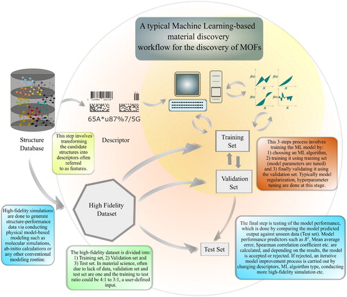
Figure 3. (Colour online) (a) Selectivity plot of Xe/Kr in the training set with RMSE data [103], (b) Feature importance plot for all descriptors, (c) Selectivity plot of Xe/Kr in the test set with RMSE data, and (d) Distribution of simulated selectivities in the diverse training set compared with a randomly selected set from the dataset. Reprinted with permission from American Chemical Society.

Figure 4. (Colour online) A DT model for the CO${}_2$ uptake capacity higher than (a) 2 mmol/g, (b) 4 mmol/g of the 32,450 MOFs in the training data set. Each branch represents a QSPR score of 1 or 0 assigned to that MOF if it satisfies a descriptor threshold criteria. The final scores below are averaged QSPR scores [48]. Reprinted with permission from European Journal of Inorganic Chemistry.

Figure 5. (Colour online) The top plot figure shows the log(frequency) with net H${}_2$ delivery capacity for all the databases [107]; while the bottom figure is the net deliverable energy versus void fraction plot. Reprinted with permission from American Chemical Society.

Figure 6. (Colour online) The table at the top shows the respective performance of different descriptors for different algorithms in terms of R${}^2$, and root mean square error (RMSE). The bottom figure shows the parity plots for ML-predicted methane uptake versus GCMC simulated data on (a) DT, (b) Poisson regression, (c) SVM, and (d) RF models. The colour scale of the right indicates number of times or number of hMOFs that had the equivalent GCMC and ML result [108]. Reprinted with permission from American Chemical Society.

Figure 7. (Colour online) Parity plots for comparing CO${}_2$ selectivity data over N${}_2$ prediction for different ML methods with respect to GCMC calculations [110]. The correlation coefficient R${}^2$ and Spearman ranking correlation coefficient (SRCC) results are also shown for each model. Reprinted with permission from American Chemical Society.

Figure 8. (Colour online) Scatter plots for Methane and CO${}_2$ uptake prediction at different pressure based on AR-RDF descriptors versus predicted via GCMC calculations of ∼25000 MOF structures [119]. The correlation coefficient R${}^2$ is shown for all the cases. All the calculation are done at industrial pressure swing adsorption (PSA) conditions. Reprinted with permission from American Chemical Society.

Figure 9. (Colour online) The workflow for generating energy descriptor for hydrogen storage [133]. The procedure begins with sampling the potential energy distribution of H${}_2$-MOF interaction in multiple even spaced grid, followed by binning those energy in a histogram. Each of the bins then form an identifier in the energy descriptor of that MOF represented by the input vector $X_i$. Reprinted with permission from American Chemical Society.

Figure 10. (Colour online) A latent representation of cages, which is simply the rows of the matrix $U_{\nu }{\mathrm{\Sigma }}_{\nu }$ – which is an equivalent form of Equation (6(6) $\mathrm{R}\mathrm{S}\mathrm{S}=\sum _{i=1}^n\parallel X_i-\sum _{j=1}^k{\alpha }_{ij}{Z}_i{\parallel }^2$(6) )'s right hand side term $U_{\nu }{\mathrm{\Sigma }}_{\nu }\equiv {\sigma }_i{u}_i\left[k\right]$ – embedded into 2D by t-SNE [134]. The coloured points shows the simulated Xe/Kr selectivity of an isolated cage structure at 298 K in an empty box. Furthermore, the points nearby are nearer to each other in the latent cage space and thus are likely to exhibit similar Xe/Kr selectivity while cages marked ‘X’ have too small a window for xenon to enter into the cavity. Reprinted with permission from ACS (American Chemical Society). Further permissions related to the material excerpted should be directed to the ACS.

Table 3. A list of some more second-order descriptors with applications and material class.

Descriptor	Properties of interest	Material class	Year
Channel factor and perpendicular	Thermal transport properties	Porous media	2020 [136]
non-uniformity
Local porosity and local mean	Shortest transportation paths	porous materials	2020 [137]
geodesic tortuosity
Geometric landscape within energy–	Gas adsorption	Porous materials	2020 [138]
structure–function(ESF) maps
Persistent homology-based	CH${}_4$ Adsorption	Zeolites	2020 [139]
topological descriptors
PES of the MOF with a probe	CH${}_4$ Adsorption	MOFs	2019 [140]
atom of radius a
Experimentally derived specific	Electric double-layer (EDL)	Nanoporous carbons	2019 [141]
surface area and volume	Capacitance	Material
Fraction of pore size
Pore geometry barcode-based	CH${}_4$ Adsorption	Nanoporous materials	2019 [142]
descriptors: set of distances
from the structure to the most
diverse set in the barcode, and
most important feature of the barcode
Property-labelled materials fragments	Band gap energy,	Inorganic crystals	2017 [143]
	Bulk/shear moduli, Debye
	Temperature, metal/insulator
	Classification and heat capacities
Position of s orbital, number of	CO and NO adsorption	Zeolites	2017 [144]
valence electrons of the active
site and the HOMO-LUMO (highest
occupied molecular orbital and lowest
unoccupied molecular orbital) gap of
the adsorbate
Van der waals surface area	Propensity for structural voids,	Crystalline materials	2016 [145]
	Degree of porosity
Pore landscape descriptors: pore size	Similarity among structures	Crystalline porous	2013 [146]
distribution and stochastic rays		Materials

Omar KF, Ibrahim E, Nak Cheon J, et al. Metal-Organic framework materials with ultrahigh surface areas: is the sky the limit? J Am Chem Soc. 2012;134(36):15016–15021.

 PubMed Web of Science ®Google Scholar

Furukawa H, Ko N, Go YB, et al. Ultrahigh porosity in metal-organic frameworksScience. 2010;329:424–428.

 PubMed Web of Science ®Google Scholar

Farha OK, Yazaydın AO, Eryazici I, et al. De novo synthesis of a metal-organic framework material featuring ultrahigh surface area and gas storage capacitiesNat Chem. 2010;2:944–948.

 PubMed Web of Science ®Google Scholar

Koh K, Wong-Foy AG, Matzger AJ. A porous coordination copolymer with over 5000 m 2/g BET surface areaJ Am Chem Soc. 2009;131:4184–4185.

 PubMed Web of Science ®Google Scholar

Yan Y, Telepeni I, Yang S, et al. Metal-Organic polyhedral frameworks: high H 2 adsorption capacities and neutron powder diffraction studiesAm Chem Soc. 2010;132:4092–4094.

 PubMed Web of Science ®Google Scholar

Klein N, Senkovska I, Baburin IA, et al. Route to a family of robust, non-interpenetrated metal-organic frameworks with pto-like topologyChem Eur J. 2011;17:13007.13016

 PubMed Web of Science ®Google Scholar

Furukawa H, Miller MA, Yaghi OM. Independent verification of the saturation hydrogen uptake in MOF-177 and establishment of a benchmark for hydrogen adsorption in metal-organic frameworksJ Mater Chem. 2007;17:3197.

 Web of Science ®Google Scholar

An J, Farha OK, Hupp JT, et al. Metal-adeninate vertices for the construction of an exceptionally porous metal-organic frameworkNat Commun. 2012;3:604.

 PubMed Web of Science ®Google Scholar

Ferey G, Mellot-Draznieks C, Serre C, et al. A chromium terephthalate-based solid with unusually large pore volumes and surface areaScience. 2005;309:2040.2042

 PubMed Web of Science ®Google Scholar

Koh K, Wong-Foy AG, Matzger A. A porous coordination copolymer with over 5000 m 2/g BET surface area. J Angew Chem Int Ed. 2008;47:677.

 PubMed Web of Science ®Google Scholar

Sumida K, Hill MR, Horike S, et al. Synthesis and hydrogen storage properties of Be12 (OH) 12 (1, 3, 5-benzenetribenzoate) 4. J Am Chem Soc. 2009;131:15120.

 PubMed Web of Science ®Google Scholar

Zhao D, Yuan D, Sun D, et al. Stabilization of metal-organic frameworks with high surface areas by the incorporation of mesocavities with microwindows. J Am Chem Soc. 2009;131:9186.

 PubMed Web of Science ®Google Scholar

Dey C, Kundu T, Biswal BP, et al. Crystalline metal-organic frameworks (MOFs): synthesis, structure and function. Acta Crystallogr B Struct Sci Cryst Eng Mater. 2014 Feb;70(Pt 1):3–10. DOI: 10.1107/S2052520613029557. Epub 2013 Dec 10. PMID: 24441122.

 PubMedGoogle Scholar

Aghaji MZ, Fernandez M, Boyd PG, et al. Quantitative structure-property relationship models for recognizing metal organic frameworks (MOFs) with high CO2 working capacity and CO2/ CH4 selectivity for methane purification. Eur J Inorg Chem. 2016;2016:4505–4511.

 Google Scholar

Chung YG, Haldoupis E, Bucior BJ, et al. Advances, updates, and analytics for the computation-ready, experimental metal-organic framework database: CoRE MOF 2019. J Chem Eng Data. 2019;64(12):5985–5998.

 Web of Science ®Google Scholar

Wilmer CE, Leaf M, Lee CY, et al. Large-scale screening of hypothetical metal-organic frameworks. Nat Chem. 2011 Nov 6;4(2):83–89.

 PubMed Web of Science ®Google Scholar

Moghadam PZ, Li A, Liu XW, et al. Targeted classification of metal-organic frameworks in the Cambridge structural database (CSD). Chem Sci. 2020; 11(32):8373–8387. Advance Article

 PubMed Web of Science ®Google Scholar

Bao Y, Martin RL, Haranczyk M, et al. In silico prediction of MOFs with high deliverable capacity or internal surface area. Phys Chem Chem Phys. 2015 May 14;17(18):11962–11973.

 PubMed Web of Science ®Google Scholar

Bao Y, Martin RL, Simon CM, et al. In silico discovery of high deliverable capacity metal-organic frameworks. J Phys Chem C. 2015;119(1):186–195.

 Web of Science ®Google Scholar

Gomez-Gualdron DA, Gutov OV, Krungleviciute V, et al. Computational design of metal-organic frameworks based on stable zirconium building units for storage and delivery of methane. Chem Mater. 2014;26(19):5632–5639.

 Web of Science ®Google Scholar

Martin RL, Lin LC, Jariwala K, et al. Mail-order metal-organic frameworks (MOFs): designing isoreticular MOF-5 analogues comprising commercially available organic molecules. J Phys Chem C. 2013;117(23):12159–12167.

 Web of Science ®Google Scholar

Simon CM, Mercado R, Schnell SK, et al. What are the best materials to separate a xenon/krypton mixture?. Chem Mater. 2015;27(12):4459–4475.

 Web of Science ®Google Scholar

Thornton AW, Simon CM, Kin J, et al. Materials genome in action: identifying the performance limits of physical hydrogen storage. Chem Mater. 2017;29(7):2844–2854.

 PubMed Web of Science ®Google Scholar

Pardakhti M, Moharreri E, Wanik D, et al. Machine learning using combined structural and chemical descriptors for prediction of methane adsorption performance of metal organic frameworks (MOFs). ACS Comb Sci. 2017;19(10):640–645.

 PubMed Web of Science ®Google Scholar

Anderson R, Rodgers J, Argueta E, et al. High-throughput computational screening of metal-organic frameworks for thiol capture. Chem Mater. 2018;30(18):6325–6337.

 Google Scholar

Fernandez M, Trefiak NR, Woo TK. Atomic property weighted radial distribution functions descriptors of metal-organic frameworks for the prediction of gas uptake capacity. J Phys Chem C. 2013;117(27):14095–14105.

 Web of Science ®Google Scholar

Bucior BJ, Bobbitt NS, Islamoglu T, et al. Energy-based descriptors to rapidly predict hydrogen storage in metal-organic frameworks. Mol Syst Des Eng. 2019;4:162–174.

 Web of Science ®Google Scholar

Sturluson A, Huynh MT, York AHP, et al. Eigencages: learning a latent space of porous cage molecules. ACS Cent Sci. 2018;4(12):1663–1676.

 PubMed Web of Science ®Google Scholar

Wei H, Bao H, Ruan X. Machine learning prediction of thermal transport in porous media with physics-based descriptors. Int J Heat Mass Transf. 2020;160:120176. ISSN 0017-9310

 Web of Science ®Google Scholar

Neumann M, Machado Charry E, Zojer K, et al. On variability and interdependence of local porosity and local tortuosity in porous materials: a case study for sack paper. Methodol Comput Appl Probab. 2020; 1–15. Available from: https://doi.org/10.1007/s11009-019-09761-1:

 Web of Science ®Google Scholar

Moosavi SM, Xu H, Chen L, et al. Geometric landscapes for material discovery within energy-structure-function maps. Chem Sci. 2020;11:5423–5433.

 PubMed Web of Science ®Google Scholar

Krishnapriyan AS, Haranczyk M, Morozov D. Topological descriptors help predict guest adsorption in nanoporous materials. J Phys Chem C. 2020;124(17):9360–9368.

 Web of Science ®Google Scholar

Fanourgakis GS, Gkagkas K, Tylianakis E, et al. A robust machine learning algorithm for the prediction of methane adsorption in nanoporous materials. J Phys Chem A. 2019;123(28):6080–6087.

 PubMed Web of Science ®Google Scholar

Käärik M, Arulepp M, Käärik M, et al. Characterization and prediction of double-layer capacitance of nanoporous carbon materials using the quantitative nano-structure-property relationship approach based on experimentally determined porosity descriptors. Carbon. 2020;158:494–504.

 Web of Science ®Google Scholar

Zhang X, Cui J, Zhang K, et al. Machine learning prediction on properties of nanoporous materials utilizing pore geometry barcodes. J Chem Inf Model. 2019;59(11):4636–4644.

 PubMed Web of Science ®Google Scholar

Isayev O, Oses C, Toher C, et al. Universal fragment descriptors for predicting properties of inorganic crystals. Nat Commun. 2017;8:15679. Available from: https://doi.org/10.1038/ncomms15679

 PubMed Web of Science ®Google Scholar

Evans JD, Huang DM, Haranczyk M, et al. Computational identification of organic porous molecular crystals. CrystEngComm. 2016;18:4133–4141.

 Web of Science ®Google Scholar

Goltl F, Müller P, Uchupalanun P, et al. Developing a descriptor-based approach for CO and NO adsorption strength to transition metal sites in zeolites. Chem Mater. 2017;29(15):6434–6444.

 Web of Science ®Google Scholar

Pinheiro M, Martin RL, Rycroft CH, et al. Characterization and comparison of pore landscapes in crystalline porous materials. J Mol Graphics Model. 2013;44:208–219. ISSN 1093-3263.

 PubMed Web of Science ®Google Scholar