The importance of reference frame for pressure at the liquid–vapour interface

Figures & data

Figure 1. (Colour online) A schematic showing a single control volume and the action of the different mathematical terms in the SF expression. The location of a surface crossing, ${\lambda }_k$, is checked to be between the two molecules using the difference $H(1-{\lambda }_k)-H(-{\lambda }_k),$ while the various Λ expressions act to limit the crossing to within a rectangular region of the surface. The normal at the point of crossing is used in the calculation of the surface term. The top right shows different example contours between molecules including the Irving Kirkwood as a solid line and two interpretations of the Harasima as different dotted lines assumed to move tangentially to the surface until it gets to a line either normal (which is consistent with the definition but can have multiple solutions for an arbitrary surface) or along the z-axis.

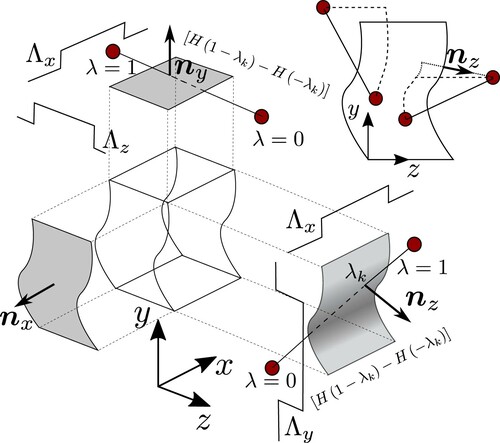
Figure 2. (Colour online) A schematic of the three cases considered in this work: (a) a solid-liquid interface with a fixed grid, (b) a liquid–vapour interface with a fixed grid and (c) a liquid–vapour interface with a grid moving with the intrinsic interface. The profiles of normal pressure are shown below with kinetic (

), configurational (

) and total (

) pressure contributions.

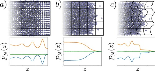
Figure 3. (Colour online) Comparing wall-normal, $P_N$, pressure measurements near a solid–liquid interface showing (a) half channel and (b) near-wall region. The kinetic components are shown for IK1 (

), VA (

) and SF (

), the configurational part for IK1 (

), VA (

) and SF (

) while the total pressure is IK1 (

), VA (

) and SF (

). The density (

) with the zero axis shown by a horizontal black line (

) and the shaded region on (a) is the section shown in (b).

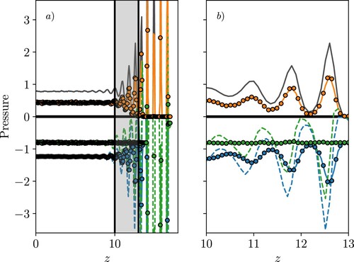
Figure 4. (Colour online) (a) Normal $P_N$ and (b) tangential $P_T$ pressure near a liquid–vapour interface using a fixed reference frame (a uniform grid). The kinetic components for IK1 (

), VA (

) and SF (

), the configurational part for IK1 (

), VA (

) and SF (

) and the total pressure for IK1 (

), VA (

) and SF (

) with the zero axis shown by a horizontal black line (

). The Irving Kirkwood contour would give the same normal and tangential pressure as the VA and SF curves.

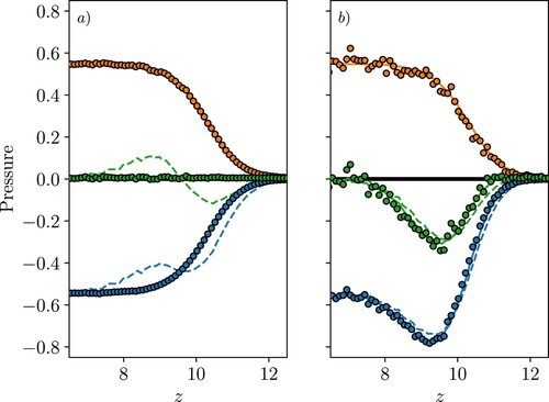
Figure 5. (Colour online) (a) Normal $P_N$ and (b) tangential $P_T$ pressure for a reference moving with the liquid–vapour interface, showing the kinetic components for IK1 (

), VA (

) and SF (

) (note the dashed line exactly follows the solid line) and the configurational part for IK1 (

), VA (

) and SF (

) with density (

) with the zero axis shown by a horizontal black line (

). The Harasima contour would give the same normal pressure as the SF curves in (a) and the same tangential pressure as the IK1 in (b).

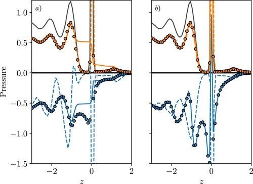
Figure 6. (Colour online) The total pressure components for a reference moving with the interface: (a) normal $P_N$ and (b) tangential $P_T$, with IK1 (

), VA (

) and SF (

) with the kinetic and configurational constituent parts from Figure 5 shown faintly for reference and zero axis shown by a horizontal black line (

). The Harasima contour would give the same normal pressure as the SF curves in (a) and same tangential pressure as the IK1 in (b).

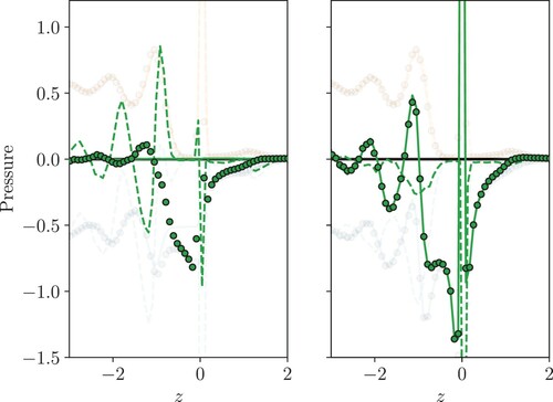
Figure 7. (Colour online) The cumulative integral of the total pressures in a reference moving with the interface shown in Figure 6 with normal $P_N$ on (a) and the negative of the tangential $-P_T$ pressure shown on (b), starting from z=−5 up to the current z on the axis, for the IK1 (

), VA (

) and SF (

) measurements, and the horizontal black line (

) is the zero axis. The inserts zoom in on the values that the integrals have converged to by the upper limit displayed on the plot, z=2, where the sum of normal and tangential components would give the total surface tension.

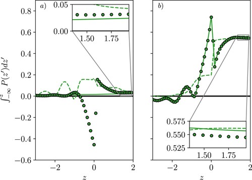
Figure 8. (Colour online) The terms required to balance normal pressure in a reference moving with the interface, where (a) shows the normal component of the Volume Average (VA) pressure, both kinetic (

) and configurational (

) with additional correction terms from Equations (26(26) $\begin{array}{rl}& \sum _{i=1}^N{m}_i{\dot{r}}_i\frac{\mathrm{d}{\vartheta }_i}{\mathrm{d}t}=\\ & \frac{\mathrm{\partial }}{\mathrm{\partial }\mathbf{r}}\cdot \stackrel{\stackrel{VA}{P}k\mathrm{\Delta }V}{\overbrace{\sum _{i=1}^N{m}_i{\dot{r}}_i{\dot{r}}_i{\vartheta }_i}}+\stackrel{\text{Extra Kinetic Curvature }\left(\mathrm{K}\mathrm{C}\right)\text{ Terms}}{\overbrace{\sum _{i=1}^N{m}_i{\dot{r}}_i{\dot{r}}_i\cdot \left[\frac{\mathrm{\partial }{\xi }_i^{+}}{\mathrm{\partial }{\mathbf{r}}_i}\mathrm{d}{S}_{zi}^{+}-\frac{\mathrm{\partial }{\xi }_i^{-}}{\mathrm{\partial }{\mathbf{r}}_i}\mathrm{d}{S}_{zi}^{-}\right]}}\\ & +\underset{\text{Extra Time Evolving }\left(\mathrm{T}\mathrm{E}\right)\text{ Terms}}{\underbrace{\sum _{i=1}^N{m}_i{\dot{r}}_i\left[\frac{\mathrm{\partial }{\xi }_i^{+}}{\mathrm{\partial }t}\mathrm{d}{S}_{zi}^{+}-\frac{\mathrm{\partial }{\xi }_i^{-}}{\mathrm{\partial }t}\mathrm{d}{S}_{zi}^{-}\right]}}\end{array}$(26) ) and (27(27) $\begin{array}{rl}\sum _{i,j}^N{\mathbf{f}}_{ij}{\mathbf{r}}_{ij}\cdot \underset{0}{\overset{1}{\int }}\frac{\mathrm{\partial }{\vartheta }_{\lambda }}{\mathrm{\partial }{\mathbf{r}}_{\lambda }}\mathrm{d}\lambda & =-\frac{\mathrm{\partial }}{\mathrm{\partial }\mathbf{r}}\cdot \stackrel{\stackrel{VA}{P^C}\mathrm{\Delta }V}{\overbrace{\sum _{i,j}^N{\mathbf{f}}_{ij}{\mathbf{r}}_{ij}\underset{0}{\overset{1}{\int }}{\vartheta }_{\lambda }\mathrm{d}\lambda }}\\ & +\underset{\text{Extra Configurational Curvature }\left(\mathrm{C}\mathrm{C}\right)\text{ Term}}{\underbrace{\sum _{i,j}^N{\mathbf{f}}_{ij}{\mathbf{r}}_{ij}\cdot \underset{0}{\overset{1}{\int }}\left[\frac{\mathrm{\partial }{\xi }_{\lambda }^{+}}{\mathrm{\partial }{\mathbf{r}}_{\lambda }}\mathrm{d}{S}_{z\lambda }^{+}-\frac{\mathrm{\partial }{\xi }_{\lambda }^{-}}{\mathrm{\partial }{\mathbf{r}}_{\lambda }}\mathrm{d}{S}_{z\lambda }^{-}\right]\mathrm{d}\lambda }},\end{array}$(27) ) including kinetic curvature $\mathrm{\partial }{\xi }_i/\mathrm{\partial }{\mathit{r}}_i$, KC, (

), time-evolving $\mathrm{\partial }{\xi }_i/\mathrm{\partial }t$, TE, (

) as well as the negative of the configurational curvature $\mathrm{\partial }{\xi }_{\lambda }/\mathrm{\partial }{\mathit{r}}_{\lambda }$, CC, (

) (shown as negative to allow comparison with the VA configurational pressure). In figure (b), the VA pressure is displayed with the correction terms added compared to the SF forms, which naturally include all of these terms. These include the kinetic VA with KC and TE added (

) compared to kinetic SF (

), configurational VA with CC added (

) against configurational SF (

) and total corrected VA (

) against total SF (

). The zero axis is shown by a horizontal black line (

).

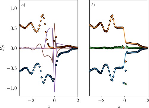
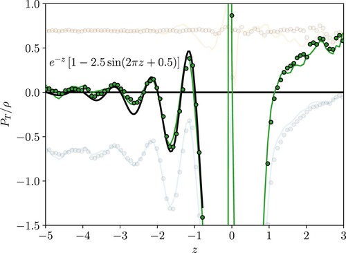
Figure 9. (Colour online) Total tangential pressure divided by density for quantities in a reference frame moving with the interface, VA (

) and total SF (

). The kinetic, SF (

), VA (

), and configurational, SF (

), VA (

) components are shown faintly in the background for reference. A fitting is shown (

) with functional form and fitting coefficients annotated on the figure with the zero axis the horizontal black line (

).

Data Availability

The data that support the findings of this study are freely available from https://doi.org/10.24435/materialscloud:5b-0g saved in the open Python pickle format with all required Python scripts to load the data and reproduce the figures in this work (as well as allowing further analysis of the data). The input files to simulate this exact case are also included in the above link with a README.txt explaining the process of building and running Flowmol. The latest version of the Flowmol code is freely available from https://github.com/edwardsmith999/flowmol, however, to ensure reproducibility, the version of Flowmol used to generate the data in this work is available at the following persistent link https://doi.org/10.5281/zenodo.4639546.