The impact of the thermostats on the non-equilibrium computer simulations of the interfacial thermal conductance

Figures & data

Table 1. Simulation parameters used in this work for gold and water.

Non-bonded parameters	ϵ [kcal mol${}^{-1}$]	σ [Å]	q [e]	m (g/mol)
Au${}_c$	3.50	2.6246	+1.0	195.967
Au${}_s$	0.20	2.6246	−1.0	1.00
O	0.15535	3.166	−0.8476	15.9994
H	0.0	0.0	+0.4238	1.00794

Note: Au${}_c$ and Au${}_s$ represent the core and shell sites defining the gold atoms.

Figure 1. (Colour online) Normalised heat flux correlation function of gold, considering all the atoms, core and shell particles (yellow), core particles only (green), or shell paricles only (red, shifted by -0.5). The inset shows the integrals given by Equation (5(5) ${\tau }_{J_q}={\int }_0^{t_{max}}\frac{⟨{\mathbf{J}}_q(t^{\prime })\cdot {\mathbf{J}}_q(0)⟩}{⟨{\mathbf{J}}_q(0)\cdot {\mathbf{J}}_q(0)⟩}\mathrm{d}{t}^{\prime }$(5) ). The dashed lines correspond to the secondary y-axis. The relaxation times are 0.027 ps, 0.037 ps, 1.42 ps, for shell particles, all particles and core particles, respectively.

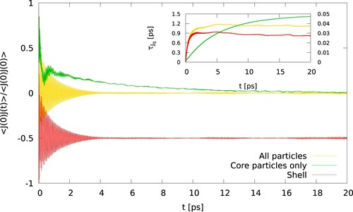
Figure 2. (Colour online) Interfacial density profile of water as a function to the distance to the gold surface. The green-shaded area represents the region used to select water molecular for the calculation of the interfacial vibrational density of states. The inset shows the number of atoms (hydrogens and oxygens) that were initially in the interfacial region, and that stay in that region after time t. After 4 ps (the correlation time for Equation (6(6) $D_{\alpha ,\xi }(\omega )={\int }_0^{\mathrm{\infty }}\frac{⟨v_{\alpha ,\xi }(0)v_{\alpha ,\xi }(t)⟩}{⟨v_{\alpha ,\xi }(0)v_{\alpha ,\xi }(0)⟩}\exp (-2\pi i\omega t)\mathrm{d}t$(6) )), ∼90% of the original water molecules remain in the interfacial region. The full line corresponds to the average of 10 individual trajectories (shown by the dotted lines light blue).

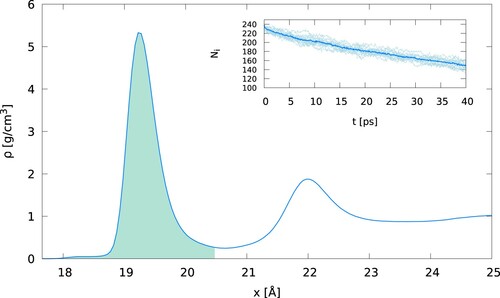
Figure 3. (Colour online) Energy exchanged in the hot (red) and cold (blue) thermostats, for Langevin (left) and canonical velocity rescaling (right). The timestep is $\delta t=0.5\mathrm{fs}$, and the thermostats damping time is ${\tau }_D=0.1\mathrm{ps}$ (top panels) or ${\tau }_D=2.5\mathrm{ps}$ (bottom panels). We have changed the sign of the $E_{cold}$ to faciliate the comparison of both sets of data.

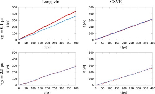
Figure 4. (Colour online) Heat rate difference between the hot and cold thermostats for Langevin (left) and canonical velocity rescaling (right), as a function of the damping time, ${\tau }_D$, for different integration timesteps $\delta t$.

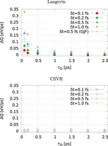
Figure 5. (Colour online) Temperature profiles obtained using the Langevin or CSVR thermostats with a damping time ${\tau }_D=0.1\mathrm{ps}$ (top) or ${\tau }_D=2.5$ (bottom). Both thermostats are applied to all the particles (core and shell) in the gold slab. For all the panels, the empty symbols represent the temperatures of the core or shell atoms, highlighting their temperature differences.‘Gold’ refers to the average temperature obtained using the temperatures of the core and shell particles. The arrows signal the interfacial region used to calculate the temperature jump.

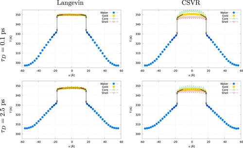
Figure 6. (Colour online) Thermal conductance for Langevin (top) and canonical velocity rescale (bottom) thermostats, as a function of the thermostat damping time. The thermal conductance was computed using the average of the energy exchanged in the hot and cold thermostats (filled points), or just the cold thermostat (empty points).

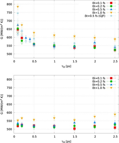
Table 2. Thermal conductances obtained in this work using different thermostats and damping constants.

		G [MW/(m${}^2$ K)]
$\delta t$ [fs]	${\tau }_D$ [ps]	Langevin	CSVR
0.5	0.1	$674\pm 10$ ($619\pm 10$)	$536\pm 8$ ($535\pm 8$)
0.5	2.5	$542\pm 10$ ($539\pm 11$)	$536\pm 14$ ($538\pm 14$)

Note: The results in parenthesis were obtained using the heat flux obtained from the energy exchanged at the cold thermostat only. The other results were obtained using the average of the heat fluxes of the cold and hot thermostat.

Figure 7. (Colour online) Vibrational density of states for the core (green) and shell (red) particles, and water (blue), using the Langevin thermostat with ${\tau }_D=2.5\mathrm{ps}$ for the gold slab. Individual components are shown with dashed (component parallel to heat flux) and dotted (component perpendicular to heat flux) lines. The total VDOS is calculated as the sum the three components, x, y and z. The VDOS of water shows significant overlap with both the core and shell particles.

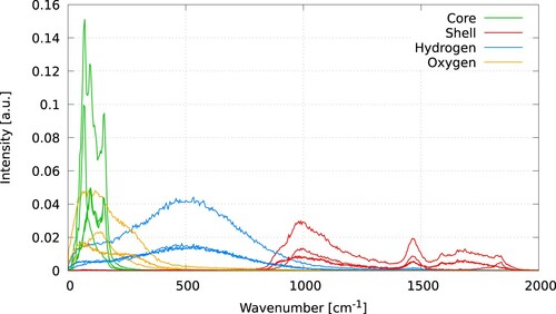
Figure 8. (Colour online) VDOS of the interfacial region, for the core (top) and shell (bottom) particles. The left (right) panels correspond to Langevin (CSVR) thermostats with different damping parameters.⁣⁣⁣⁣⁣⁣⁣

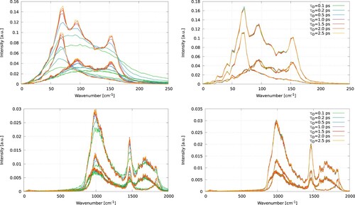
Figure 9. (Colour online) Interfacial thermal conductance as a function of the VDOS overlap, S, between different atomic species. The calculations correspond to the Langevin thermostat applied to the gold atoms (core and shell). The heat flux has been calculated using the energy exchanged in both thermostats (filled symbols), or just the water thermostat (open symbols).

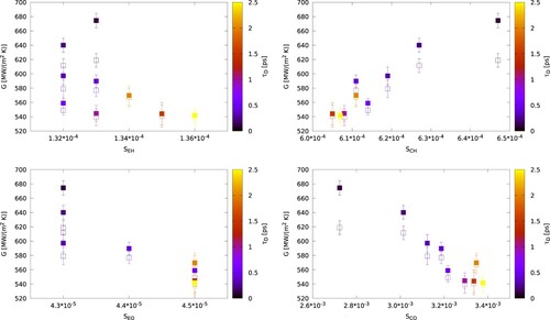
Figure 10. (Colour online) Temperature profile using the dual CSVR thermostat with ${\tau }_D=2.5\mathrm{ps}$ and $\delta t=0.5\mathrm{fs}$.

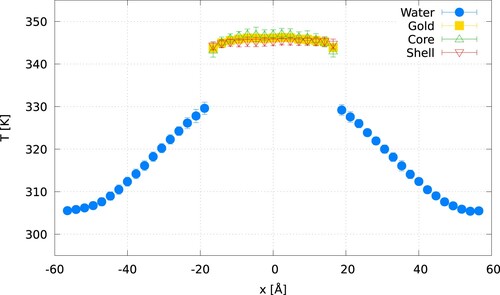
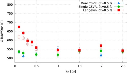
Figure 11. (Colour online) Comparison of the interfacial thermal conductance obtained with the 3 different thermostatting configurations. All the results were obtained with $\delta t=0.5\mathrm{fs}$.