Figures & data
Figure 1. (Colour online) Conservation analysis of amino acid residues in NLRC4 using ConSurf. The colour intensity reflects the degree of conservation. The Q657 amino acid (as indicated in the red box) is conserved and located in the exposed region of the protein.
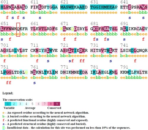
Table 1. Physicochemical properties of glutamine and leucine.
Table 2. The pathogenicity prediction of Q657L mutation in NLRC4 using in silico prediction tools.
Figure 2. (Colour online) Graph of RMSD values as a function of time and superposition of wild-type structure with the mutant structure. (a) Black denotes wild-type structure and red denotes mutant structure in the resting state. (b) Blue denotes wild-type structure and green denotes mutant structure in the activated state. The reference structures for the wild-type and mutant (at 0 ns) were the energy-minimised homology models. The simulations of all structures reached local equilibrium during 65–100 ns of simulation. The conformations of the mutant structures were different from the wild-type structures at a specific time point.
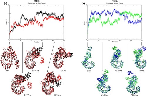
Figure 3. (Colour online) Graph of RMSF values of Cα atoms as a function of amino acids and predicted secondary structures of the average structures. (a) Cα atoms RMSF analysis of wild-type and mutant structure in the resting state (top). Black denotes wild-type structure and red denotes mutant structure in the resting state. Schematic wiring diagrams (bottom) show the secondary structure of the average structure (from 65 to 100 ns MD simulation). The purple diagram denotes wild-type average structure in the resting state; the red diagram denotes average mutant structure in the resting state. Strands are represented by arrows, and helices are represented by strings. (b) Cα atoms RMSF analysis of wild-type and mutant structure in the activated state (top). Blue denotes wild-type structure and green denotes mutant structure in the activated state. The schematic wiring diagram (bottom) in blue denotes wild-type average structure in the activated state, and green diagram denotes average mutant structure in the activated state. In both states, flexibility in mutant structure was lower than wild-type structure in most residues. In resting state, residues at locations, 143–145, 147, 149, 299, 330–331, 334, 336, 378–379, 520–521, 524–529, 535–537, 542, 545–546, 549, 553, 581, 590–596, 618–636, 643, 647–650, 873, 876–877, 905–907, 998–999, 1018–1020, were more flexible in mutant structure. The mutant structure exhibited higher fluctuation at residues 145, 412–414, 521, 530, 628–639, 771–775, 780, 798–812, 826–839, 855–868, 887–891 in the activated state. Schematic diagrams show changes in the secondary structures in the region between residues 3–30, 35–43, 61–75, 89–99, 193–194, 255–257, 281–286, 519–521, 648–654, 726–734, 795–802, 858–860, and 865–877 in the wild-type and mutant structure of the resting state. Changes of the secondary structures in the region between residues 65–84, 159–160, 251–262, 282–284, 288–290, 408–410,534–538, 602–608, 610–617, 795–801, 809–815, 859–860, and 888–889 were observed in the wild-type and mutant structure of the activated state.
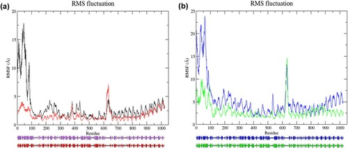
Figure 4. (Colour online) The secondary structure elements between the residues 500–700 of NLRC4 in the resting and activated state during 65–100 ns of simulation based on DSSP classification. (a) Wild-type structure in the resting state. (b) Mutant structure in the resting state. (c) Wild-type structure in the activated state. (d) Mutant structure in the activated state.
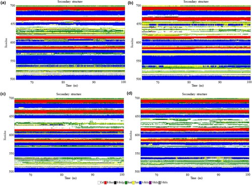
Figure 5. (Colour online) Radius of gyration (Rg) values of Cα atoms as a function of time from 65 to 100 ns of simulation. (a) Black denotes wild-type structure and red denotes mutant structure in the resting state. (b) Blue denotes wild-type structure and green denotes mutant structure in the activated state. The degree of compactness is reflected by the change in Rg value. A constant Rg value denotes no change in folding. In the resting state, the mutant structure was more stably folded than the wild-type structure in the last 35 ns of simulation. While the mutant structure was notably more compact than the wild-type structure in the activated state.
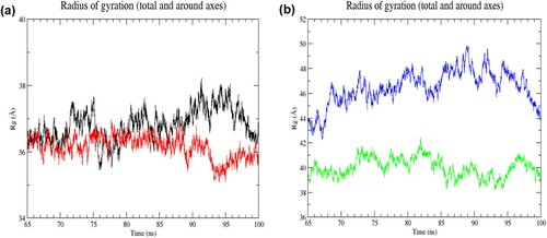
Figure 6. (Colour online) Solvent accessible surface area (SASA) of proteins as a function of time from 65 to 100 ns of simulation. (a) Black denotes wild-type structure and red denotes mutant structure in the resting state. (b) Blue denotes wild-type structure and green denotes mutant structure in the activated state. The wild-type and mutant structures in the activated state had higher SASA values than those in the resting state.
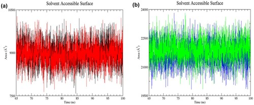
Figure 7. (Colour online) The number of intramolecular hydrogen bonds as a function of time from 65 to 100 ns of simulation. (a) Black denotes wild-type structure and red denotes mutant structure in the resting state. (b) Blue denotes wild-type structure and green denotes mutant structure in the activated state. In the resting state, more numbers of intramolecular bonds were formed in the mutant than in the wild-type structure. The mutant structure had lesser intramolecular hydrogen bonds than the wild-type structure in the activated state.
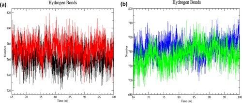
Figure 8. (Colour online) The number of intermolecular hydrogen bonds as a function of time from 65 to 100 ns of simulation. (a) Black denotes wild-type structure and red denotes mutant structure in the resting state. (b) Blue denotes wild-type structure and green denotes mutant structure in the activated state. Lesser intermolecular bonds were formed in the mutant than the wild-type structure in the resting state. The mutant structure had more intermolecular hydrogen bonds than the wild-type structure in the activated state.
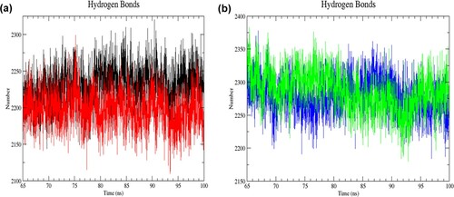
Figure 9. (Colour online) Principal component analysis of NLRC4 during the last 35 ns of simulation. (a) The plot of eigenvalues vs. eigenvector index for the first ten eigenvectors of wild-type and mutant structure in the resting state. Black denotes wild-type structure and red denotes mutant structure in the resting state. (b) Plot of eigenvalues vs. eigenvector index for the first ten eigenvectors of wild-type and mutant structure in the activated state. Blue denotes wild-type structure and green denotes mutant structure in the activated state. (c) 2D projection of the motion for wild-type and mutant structure in resting state. (d) 2D projection of the motion for wild-type and mutant structure in the activated state. In both states, both mutant structures (RM and AM) occupied a smaller region of phase space than the wild-type structures (RW and AW), indicating a decrease in the overall flexibility of mutant structures in the last 35 ns of simulations.
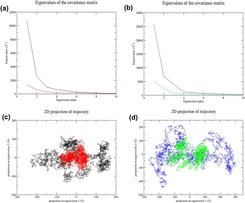
Figure 10. (Colour online) Gibbs free energy landscapes of the first two principal components (PC1 and PC2) during 65–100 ns MD simulation. The free energy value is given in kJ/mol shown by the colour bar. The blue colour region in the plot indicates lower energy. (a) Wild-type structure in the resting state. (b) Mutant structure in the resting state. (c) Wild-type structure in the activated state. (d) Mutant structure in the activated state.
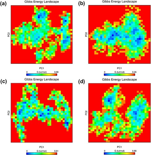
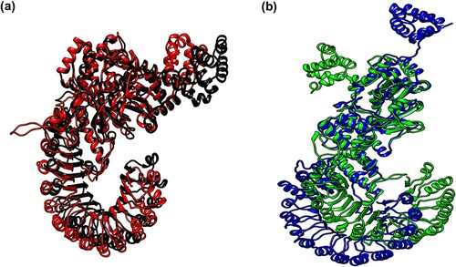
Figure 11. (Colour online) Cluster analysis of MD simulation trajectories of NLRC4 proteins. The representative structure of the top cluster obtained from the trajectories of 65–100 ns MD simulation. (a) Superposition of the representative structure of wild-type (black) and mutant (red) protein in the resting state. (b) Superposition of the representative structure of wild-type (blue) and mutant (green) protein in the activated state.