Predicting the in vitro dissolution rate constant of mineral wool fibers from fiber composition

Figures & data

Table 1. Oxide chemistry of several synthetic vitreous fibers (SVF) used in this study.

Oxide	MMVF34 (wt %)	QFHA19 (wt %)	QFHA22 (wt %)	QFHA25 (wt %)
SiO2	38.9	40.1	41.6	38.3
Al2O3	23.2	18.9	21.6	22.7
CaO	15.0	19.1	15.6	25.2
MgO	9.6	11.6	9.8	6.6
Na2O	1.9	1.8	1.7	0.7
K2O	0.8	0.5	0.4	0.4
Fe2O3	7.4	5.9	7.3	4.4
TiO2	2.1	1.6	1.7	1.2
P2O5	0.4	0.0	0.0	0.0

Notes: MMVF34 data as per reference (Barly et al. 2019). QFHA19, QFHA22, QFHA25 data as per reference (Sauer et al. 2021).

Table 2. Solution chemistry of the simulant fluids used within this work.

Oxide	EU 4.5 With citrate (ppm)	EU 4.5 Without citrate (ppm)	PSF Without citrate (ppm)	PSF With citrate (ppm)
Na^+	3552	3552	2685	2685
K^+	–	–	782	782
Ca^+2	7.9	7.9	7.91	7.91
Mg^+2	25	25	–	–
Cl^−	4500	4500	4034	4034
HCO^3−	1416	1416	–	–
${\text{PO}}_4^{3-}$	100	100	95	95
${\text{SO}}_4^{-2}$	53	53	48	48
Citrate^−1	98	–	–	98
Tartrate^−1	116	116	–	–
Lactate^−1	139	139	–	–
Pyruvate^−1	136	136	–	–
glycine^−1	118	118	444	444
H2CO	799	799	1998	1998
CH3OH	270	270	675	675
Pthalate^−1	–	–	3303	3303

Note: PSF: Stefaniak’s Phagoloysosmal Simulant Fluid.

Figure 1. Schematic of the updated optical method cell. The fibers were mounted across the slot located mid-cell. Design schematics are provided in the Supplemental Materials.

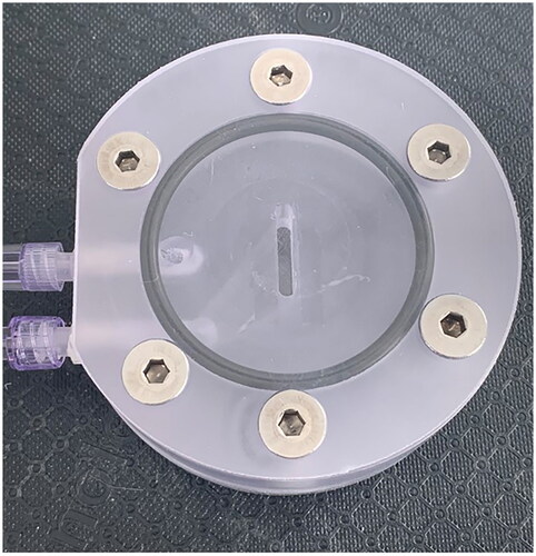
Figure 2. Typical overview of the flow cell with several fibers mounted in the fluid path (SVF: QFHA22, Fluid: PSF) with the arrows annotating single fibers.

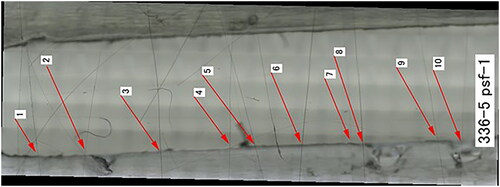
Figure 3. Typical micrographs of an individual fiber during testing. The red box represents the length over which the diameter was measured at each time step.

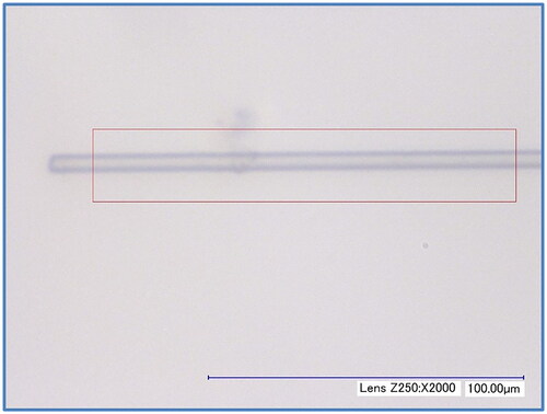
Table 3. Dissolution rate constant data from the screening experiment of QFHA19 fiber, showing significant increase in k_dis with citrate addition.

Test fluid	Citrate (mmol/L)	Kdis (ng/cm^2/hr)
EU 4.5 (no citrate)	−0-	1860 ± 1195
EU 4.5	0.52	22 288 ± 844
PSF	−0-	2165 ± 194
PSF (citrate added)	0.5	32 615 ± 3396

Note: PSF: Stefaniak’s Phagoloysosmal Simulant Fluid; K_dis: dissolution rate constant.

Table 4. Comparing measured dissolution rate constants obtained for several mineral fibers to those calculated from the Eastes model from in vivo data.

Fiber	Kdis in EU4.5 (ng/cm^2/hr)	Kdis in PSF (ng/cm^2/hr)	${\mathrm{K}}_{\text{vv}}^{\mathrm{a}}$ (ng/cm^2/hr)
MMVF34	42 474	157	698
QFHA19	22 288	2165	974
QFHA22	35 734	1008	406
QFHA25	48 481	1462	337

Note: PSF: Stefaniak’s Phagoloysosmal Simulant Fluid; K_dis: dissolution rate constant; K_vv: dissolution rate constant from in vivo biopersistence testing.

^aIn this work, we use the ‘K_vv’ nomenclature to designate a dissolution rate constant calculated from in vivo data per Eastes et al. This was done to differentiate vs. dissolution rate constants ‘K_dis’ derived from in vitro dissolution measurements.

Figure 4. The dissolution rate constant, k_dis, calculated by Equation (3)(3) $${\hspace{0.17em}\log \hspace{0.17em}\mathrm{\hspace{0.17em}}\mathrm{k}}_{\text{dis}}=\mathrm{\hspace{0.17em}}100·{\sum }_{\mathrm{i}}{\mathrm{P}}_{\mathrm{i}}·{\mathrm{W}}_{\mathrm{i}}/{\sum }_{\mathrm{i}}{\mathrm{W}}_{\mathrm{i}}$$(3) using the EU 4.5 coefficients compared to the measured value. The solid line is the ideal fit; the 80% confidence interval is an interval of x/3.9.

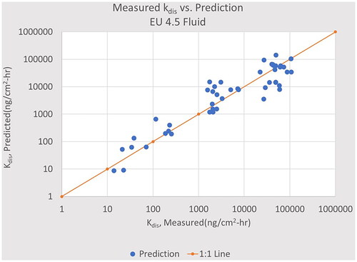
Figure 5. The dissolution rate constant, k_dis, calculated by Equation (3)(3) $${\hspace{0.17em}\log \hspace{0.17em}\mathrm{\hspace{0.17em}}\mathrm{k}}_{\text{dis}}=\mathrm{\hspace{0.17em}}100·{\sum }_{\mathrm{i}}{\mathrm{P}}_{\mathrm{i}}·{\mathrm{W}}_{\mathrm{i}}/{\sum }_{\mathrm{i}}{\mathrm{W}}_{\mathrm{i}}$$(3) using the PSF coefficients compared to the measured value. The solid line is the ideal fit; the 80% confidence interval is an interval of x/6.9. PSF, Stefaniak’s Phagoloysosmal Simulant Fluid.

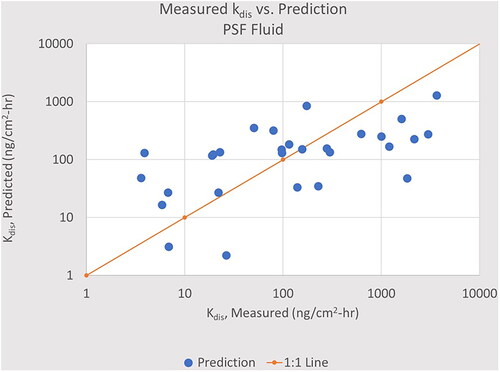
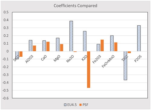
Table 5. Coefficients for the calculation of the fiber dissolution rate constant, k_dis, in EU 4.5 and PSF.

Oxide^a	EU4.5 fluid			PSF
	Coefficient, Pi	Standard error	Fiber range (wt %)	Coefficient, Pi	Standard error	Fiber range (wt %)
SiO2	−0.0989	0.0145	37.0–60.7	−0.0705	0.0399	37.0–56.5
Al2O3	0.1412	0.0137	0.5–37.0	0.0735	0.0262	0.5–25.0
CaO	0.1355	0.0091	0.0–37.5	0.1210	0.0417	15.0–34.8
MgO	0.1698	0.0330	5.0–21.0	0.0918	0.0592	5.0–20.4
Na2O	0.3861	0.1214	0.0–5.4	−0.0080	0.2601	0.0–4.0
K2O	0.2559	0.2804	0.0–1.4	−0.4677	0.2543	0.0–2.1
Fe2O3	0.0911	0.0624	0.0–6.9	0.1483	0.0751	0.4–9.3
FeO + MnO	0.2000	0.0452	0.0–7.2	0.1131	0.1093	0.3–7.5
TiO2	−0.3665	0.1568	0.0–3.0	−0.0237	0.4131	0.0–2.1
P2O5	0.3301	0.1234	0.0–5.4	–	–	–

Note: PSF: Stefaniak’s Phagoloysosmal Simulant Fluid.

^aAll oxide concentrations are as weight %.

Figure 6. Visual comparison of the coefficients by fluid, showing general agreement within the major oxides.

Barly SHQ, Okhrimenko DV, Solvang M, Yue Y, Stipp SLS. 2019. Dissolution of stone wool fibers with phenol-urea-formaldehyde binder in a synthetic lung fluid. Chem Res Toxicol. 32, 12:2398–2410.

 Web of Science ®Google Scholar

Sauer WG, Werle K, Waindok H, Hirth S, Hachmoller O, Wohlleben W. 2021. Critical choices in predicting stone wool biodurability: lysosomal fluid compositions and binder effects. Chem Res Toxicol. 34(3) :780–792.

 PubMed Web of Science ®Google Scholar

Data availability statement

All data generated or analyzed during this study are included in this published article [and its Supplementary Information Files].