Portfolio Diversification Across U.S. Gateway and Non-Gateway Real Estate Markets

Figures & data

Table 1. Sample Descriptive Statistics by Sector and Market Type.

Panel A. Beginning of Time Period (2004Q1)

	Apartment	Industrial	Office	Retail	All
# Properties
All CBSAs	399	518	521	245	1,683
Gateway	72	159	182	65	478
Non-Gateway	327	359	339	180	1,205
Aggregate Value of Properties (USD Billion)
All CBSAs	15.0	10.4	28.4	16.7	70.5
Gateway	5.0	3.6	15.9	5.4	29.9
Non-Gateway	10.0	6.8	12.5	11.3	40.5
Average Property Value (USD Million)
All CBSAs	37.5	20.1	54.6	68.0	41.9
Gateway	69.4	22.7	87.5	83.3	62.6
Non-Gateway	30.5	19.0	36.9	62.5	33.6
Capitalization Rates (%)
All CBSAs	5.20	7.30	7.07	6.98	6.69
Gateway	4.92	7.61	6.94	7.03	6.70
Non-Gateway	5.34	7.13	7.24	6.95	6.67
Spread in Capitalization Rates Between Non-Gateway and Gateway Markets (bps)
	42	−48	30	−8	−3

Panel B. End of Time Period (2019Q4)

	Apartment	Industrial	Office	Retail	All
# Properties
All CBSAs	901	1,752	710	702	4,065
Gateway	316	582	353	226	1,477
Non-Gateway	585	1,170	357	476	2,588
Aggregate Value of Properties (USD Billion)
All CBSAs	87.2	63.5	145.2	95.4	391.3
Gateway	40.1	23.4	104.8	32.1	200.4
Non-Gateway	47.2	40.1	40.4	63.3	190.9
Average Property Value (USD Million)
All CBSAs	96.8	36.2	204.5	135.8	96.3
Gateway	126.8	40.3	269.8	141.8	135.7
Non-Gateway	80.6	34.2	113.1	133.0	73.8
Capitalization Rates (%)
All CBSAs	4.25	4.48	4.26	4.60	4.37
Gateway	3.98	4.28	4.02	4.31	4.09
Non-Gateway	4.47	4.60	4.86	4.75	4.67
Spread in Capitalization Rates Between Non-Gateway and Gateway Markets (bps)
	49	32	83	44	58

Figure 1. Cumulative number of sales. Note: The figure displays the three-quarter (centered) cumulative number of true sales in the cleaned dataset.

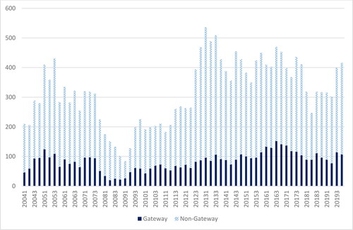
Figure 2. Ratios of sale prices to appraised values. Note: The figure depicts the median (50th percentile) of the three-quarter average of the ratio of sale price to the lagged appraised value as well as the 10th, 25th, 75th, and 90th percentiles.

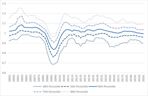
Figure 3. Portfolio and market appreciation returns. Note: The solid lines are the returns of 30 randomly selected portfolios, the dashed line is the NCREIF Property Index (NPI), and the dotted line the value-weighted NCREIF Transaction-Based Index (NTBI).

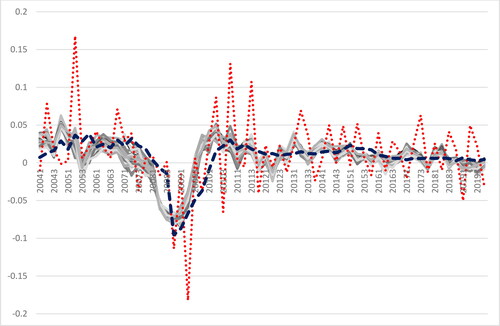
Figure 4. Distributions of portfolio total returns, standard deviations, and Sharpe ratios. Note: BC = base case, NR = quality control using NOI ratios, NRM = quality control using NOI ratios by market class, and AC = age-corrected quality control. 1.0, 0.5, and 0.0 indicate the allocation to gateway markets (100%, 50%, and 0%, respectively).

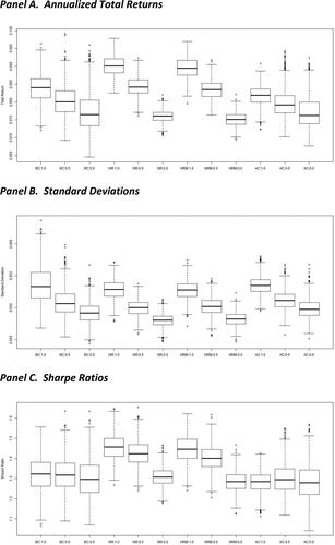
Figure 5. Distributions of annualized portfolio income and appreciation returns. Note: BC = base case, NR = quality control using NOI ratios, NRM = quality control using NOI ratios by market class, and AC = age-corrected quality control. 1.0, 0.5, and 0.0 indicate the allocation to gateway markets (100%, 50%, and 0%, respectively).

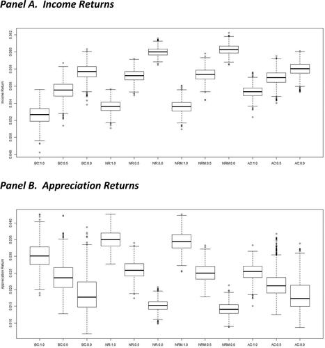
Figure 6. Portfolio downside risk measures. Note: BC = base case, NR = quality control using NOI ratios, NRM = quality control using NOI ratios by market class, and AC = age-corrected quality control. 1.0, 0.5, and 0.0 indicate the allocation to gateway markets (100%, 50%, and 0%, respectively).

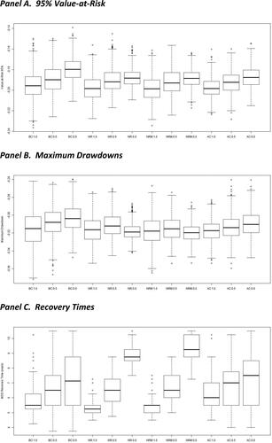
Table 2. Selected Performance Metrics for Various Sets of Gateway Markets.

	Total Returns (%)				Income Returns (%)
Gateway Weight	1.0	0.5	0.0	Δ	1.0	0.5	0.0	Δ
3 Markets	8.4	8.1	7.8	65	5.2	5.5	5.7	−48
4 Markets	8.2	8.1	7.9	29	5.3	5.5	5.7	−44
6 Markets (Base Case)	8.4	8.0	7.6	75	5.3	5.6	5.8	−50
8 Markets	8.2	8.0	7.8	49	5.3	5.6	5.8	−46
11 Markets	8.1	7.9	7.7	41	5.4	5.6	5.8	−40
	Standard Deviation of Total Returns (%)				Standard Deviation of Income Returns (%)
Gateway Weight	1.0	0.5	0.0	Δ	1.0	0.5	0.0	Δ
3 Markets	5.4	5.1	5.0	48	0.4	0.4	0.4	3
4 Markets	5.4	5.1	5.0	40	0.4	0.4	0.4	3
6 Markets (Base Case)	5.3	5.1	4.9	41	0.4	0.4	0.3	7
8 Markets	5.2	5.0	4.9	29	0.4	0.4	0.3	5
11 Markets	5.2	5.0	4.9	24	0.4	0.3	0.3	3
	Maximum Drawdown (%)				95% VaR (%)
Gateway Weight	1.0	0.5	0.0	Δ	1.0	0.5	0.0	Δ
3 Markets	−31.9	−31.0	−30.3	−167	−19.8	−19.3	−18.4	−138
4 Markets	−30.4	−30.6	−30.8	37	−18.8	−18.8	−18.8	−6
6 Markets (Base Case)	−31.5	−30.8	−30.4	−111	−19.6	−19.0	−18.0	−159
8 Markets	−31.1	−30.7	−30.4	−71	−19.3	−18.8	−18.2	−114
11 Markets	−30.7	−30.7	−30.4	−28	−19.1	−18.8	−18.3	−80

Notes: Δ denotes the spread in basis points between 100% gateway and 100% non-gateway markets. 3 Markets = New York, Los Angeles, and Chicago; 4 Markets = New York, Los Angeles, Chicago, and Washington D.C.; 6 Markets = New York, Los Angeles, Chicago, Washington D.C., Boston, and San Francisco; 8 Markets = New York, Los Angeles, Chicago, Washington D.C., Boston, San Francisco, Dallas, and Philadelphia; and 11 Markets = New York, Los Angeles, Chicago, Washington D.C., Boston, San Francisco, Dallas, Philadelphia, Atlanta, Houston, and Miami.

Figure 7. Robustness checks for sectoral composition and sectors. Note: BC = base case, CSW = constant sector weights, APT = apartments, IND = industrial, OFF = office, and RET = retail. 1.0, 0.5, and 0.0 indicate the allocation to gateway markets (100%, 50%, and 0%, respectively).

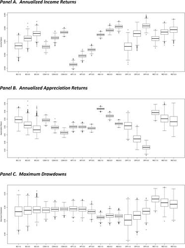
Figure 8. Composition of mixed-asset portfolios.

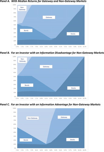
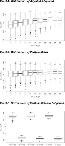
Figure 9. Distributions of adjusted R-squared and portfolio betas. Note: T1 = 2004Q1–2011Q4 and T2 = 2012Q1–2019Q4.

Panel A. Six Gateway Markets

MSA	CBSA	Div.	CBSA Name	Apart.	Ind.	Office	Retail
Boston	14460	14454	MA-Boston	G	G	G	G
Boston	14460	15764	MA-Cambridge-Newton-Framingham	G	G	G	G
Boston	14460	40484	NH-Rockingham County-Strafford County	N-G	N-G	N-G	N-G
Chicago	16980	16974	IL-Chicago-Naperville-Arlington Heights	G	G	G	G
Chicago	16980	20994	IL-Elgin	N-G	N-G	N-G	N-G
Chicago	16980	29404	IL-WI-Lake County-Kenosha County	N-G	N-G	N-G	N-G
Chicago	16980	23844	IN-Gary	N-G	N-G	N-G	N-G
Los Angeles	31080	11244	CA-Anaheim-Santa Ana-Irvine	G	G	G	G
Los Angeles	31080	31084	CA-Los Angeles-Long Beach-Glendale	G	G	G	G
New York	35620	35084	NJ-PA-Newark	N-G	N-G	G	N-G
New York	35620	20524	NY-Dutchess County-Putnam County	N-G	N-G	N-G	N-G
New York	35620	35004	NY-Nassau County-Suffolk County	N-G	N-G	N-G	N-G
New York	35620	35614	NY-NJ-New York-Jersey City-White Plains	G	G	G	G
San Francisco	41860	36084	CA-Oakland-Hayward-Berkeley	G	G	G	G
San Francisco	41860	41884	CA-San Francisco-Redwood City-South San Francisco	G	G	G	G
San Francisco	41860	42034	CA-San Rafael	N-G	N-G	N-G	N-G
Washington DC	47900	47894	DC-VA-MD-WV-Washington-Arlington-Alexandria	G	G	G	G
Washington DC	47900	43524	MD-Silver Spring-Frederick-Rockville	N-G	N-G	N-G	N-G

Note: G = Gateway; N-G = Non-Gateway.

Panel B. Additional Markets

MSA	CBSA	Div.	CBSA Name	Apart.	Ind.	Office	Retail
Atlanta	12060	12060	GA-Atlanta-Sandy Springs-Roswell	G	G	G	G
Dallas	19100	19124	TX-Dallas-Plano-Irving	G	G	G	G
Dallas	19100	23104	TX-Fort Worth-Arlington	G	G	N-G	N-G
Houston	26420	26420	TX-Houston-The Woodlands-Sugar Land	G	G	G	G
Miami	33100	22744	FL-Fort Lauderdale-Pompano Beach-Deerfield Beach	G	G	G	G
Miami	33100	33124	FL-Miami-Miami Beach-Kendall	G	G	G	G
Miami	33100	48424	FL-West Palm Beach-Boca Raton-Delray Beach	G	G	G	G
Philadelphia	37980	15804	NJ-Camden	G	G	N-G	N-G
Philadelphia	37980	33874	PA-Montgomery County-Bucks County-Chester County	G	G	G	G
Philadelphia	37980	37964	PA-Philadelphia	G	G	G	G
Philadelphia	37980	48864	DE-MD-NJ-Wilmington	N-G	N-G	N-G	N-G

Note: G = Gateway; N-G = Non-Gateway.