Bayesian design of experiments for generalized linear models and dimensional analysis with industrial and scientific application

Figures & data

Figure 1. Paper helicopter pattern.

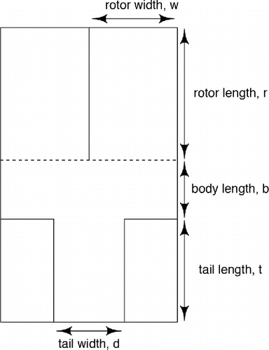
Table 1. Variable ranges and physical parameter settings (in SI units) for the paper helicopter experiment. Flight time is the measured response.

Variable/parameter (symbol)	Range/setting & units
Flight time (T)	s
Rotor width (w)	∈ [0.03, 0.09] m
Rotor length (r)	∈ [0.07, 0.12] m
Tail length (t)	∈ [0.07, 0.12] m
Mass (m)	kg
Drop height (h)	Fixed at 2  m
Acceleration due to gravity (g)	Fixed at 9.80665 ms^− 2
Air density (ρ)	Fixed at 1.20412 kgm^− 3
Paper density (D)	Fixed at 0.120 kgm^− 2
Body length (b)	Fixed at 0.025 m
Tail width (d)	Fixed at 0.05 m

Figure 2. Logistic regression example: (a) Two-dimensional projections of the SIL-optimal, pseudo-Bayesian D-optimal and central composite designs. (b) Boxplots of 20 Monte Carlo approximations of the expected self-information loss [2[2] ] using B = 20, 000 simulations for the SIL-optimal, Pseudo-Bayesian D-optimal and central composite designs.

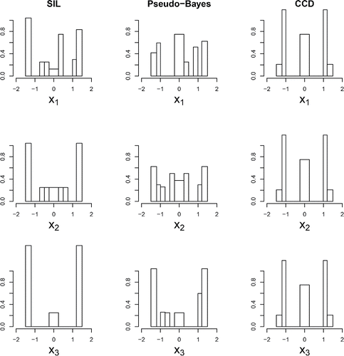
Figure 3. Logistic regression example: One-dimensional projections of the SIL-optimal, pseudo-Bayesian D-optimal, and central composite designs.

Table 2. Log-linear regression example: Minimally supported Pseudo-Bayesian D-optimal design under uniform prior distribution [8[8] ]; γ = 0.6 for α = 0.5 and γ = 0.455 for α = 0.75.

Run	x1	x2	x3	x4	x5
1	− γ	−1	1	−1	1
2	1	γ	1	−1	1
3	1	−1	− γ	−1	1
4	1	−1	1	γ	1
5	1	−1	1	−1	− γ
6	1	−1	1	−1	1

Table 3. Log-linear regression example: SIL-optimal designs under uniform prior distribution [8[8] ] for (a) α = 0.5 and (b) α = 0.75.

(a)						(b)
Run	x1	x2	x3	x4	x5	Run	x1	x2	x3	x4	x5
1	−0.500	−1	1	−1	1	1	−0.220	−1	1	−1	1
2	1	0.555	1	−1	1	2	1	0.222	1	−1	1
3	1	−1	−0.309	−1	1	3	1	−1	−0.323	−1	1
4	1	−1	1	0.334	1	4	1	−1	1	0.110	1
5	1	−1	1	−1	−0.381	5	1	−1	1	−1	−0.308
6	1	−1	1	−1	1	6	1	−1	1	−1	1

Figure 4. Log-linear regression example: Boxplots of 20 Monte Carlo approximations of the expected self-information loss [2[2] ] using B = 20, 000 simulations for the SIL-optimal and minimally supported Pseudo-Bayesian D-optimal designs (MSPBD) under uniform prior distributions [8[8] ] for (a) α = 0.5 and (b) α = 0.75.

Table 4. Helicopter experiment: (a) SEL-optimal and (b) V-optimal designs.

(a) SEL-optimal design
Run	x1	x2	x3	− log Π1
1	0.070	0.079	0.095	−1.753
2	0.070	0.087	0.102	−1.843
3	0.070	0.076	0.116	−1.769
4	0.076	0.089	0.073	−1.593
(b) V-optimal design
Run	x1	x2	x3	− log Π1
1	0.070	0.090	0.120	−1.903
2	0.070	0.090	0.120	−1.903
3	0.120	0.030	0.070	0.351
4	0.120	0.030	0.070	0.351

Figure 5. Helicopter experiment: Boxplots of 20 Monte Carlo approximations of the average expected posterior variance [3[3] ] from B = 20, 000 simulations.