
Figures & data
Figure 1. Contingency matrix. The figure reports the four possible cases for default signaling. The rows of the contingency matrix correspond to the true class and the columns correspond to the predicted class. Diagonal and off-diagonal cells correspond to correctly and incorrectly classified observations, respectively.
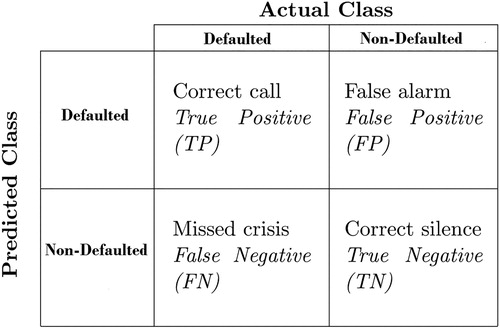
Table 1. Summary statistics of the original dataset.
Table 2. Summary statistics the transformed dataset.
Figure 2. Minimal spanning tree representation of the borrowing companies networks. The tree has been obtained by using the Euclidean distance between companies, based on the available 11 financial ratios institutions features and the Prim algorithm. Nodes are colored according to their financial soundness, red nodes represent defaulted institutions while green nodes are associated with active companies. Notice how defaulted institutions strongly occupy certain specific communities not being equally distributed among the networks.
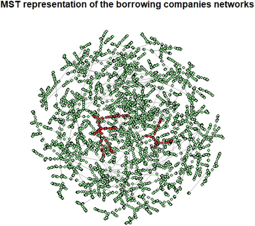
Figure 3. Correlation network based on the asset turnover.
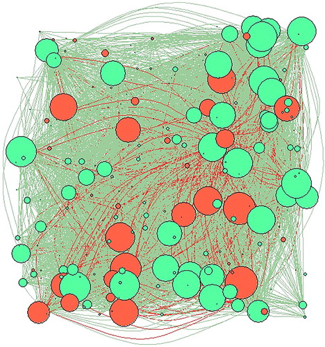
Figure 4. Correlation network based on the leverage.
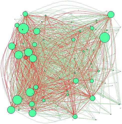
Figure 5. Correlation network based on the return on equity. Number of nodes = 226.
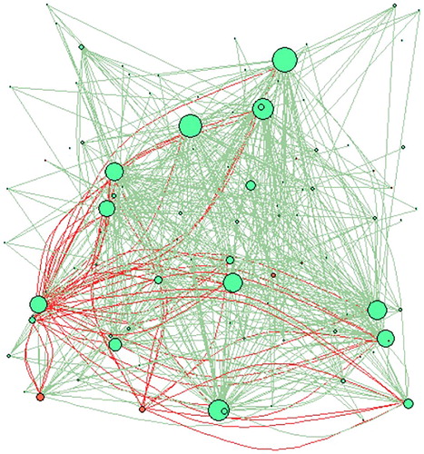
Figure 6. Centrality measure distributions. The panels represent the distribution of the centrality measures separated according to the defaulted indicator γ, together with the corresponding power-law coefficient estimate. In the left panels, we represent the degree distributions, the central panels refer to the strength distributions while the right panels encompass the PageRank distributions. The different values of the scaling coefficients related to the distributions of defaulted and active institutions suggest their potential value for discriminating between such companies.
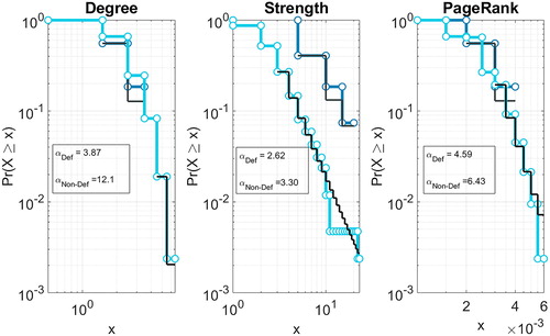
Table 3. Estimation results.
Figure 7. Model comparison. The panels represent the comparison of the predictive performance of the three models considered taking into account the receiver operating characteristic curve for all three trained classifiers. Specifically, we represent the predictive performance of: (i) the logit classifier taking into account all available variables (black line), (ii) the logit classifier taking into account variables obtained through a stepwise selection and (iii) logit classifier taking into account variables obtained through a stepwise selection and the network parameters obtained from the MST representation of borrower companies.
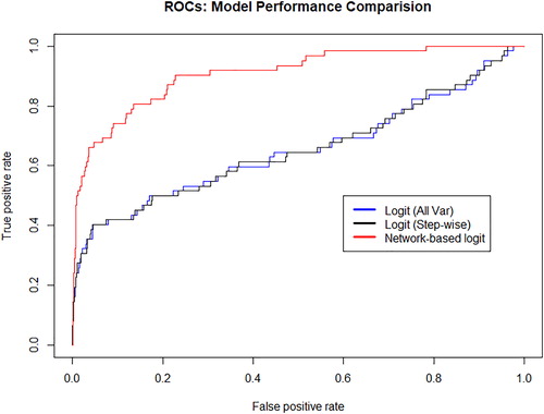
Figure 8. Precision Recall (PR) curves for the baseline credit risk models and for the network-augmented models. In the panel, similarly as in , the blue line represents the precision-recall curve for the logit regression with all variables; the black line represents the precision-recall curve for the logistic regression with variables selected through step-wise and the red line represents the precision-recall for the network augmented regression.
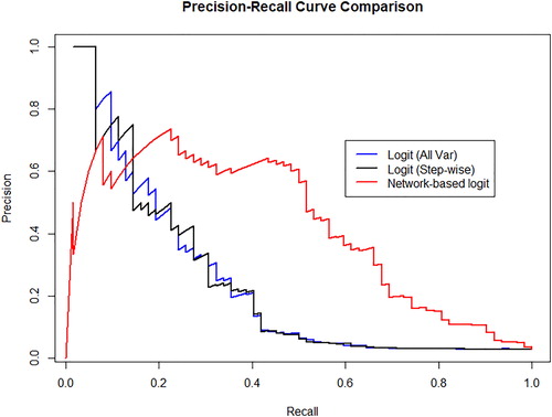
Table 4. PD estimations of the three classifiers: (i) PD from baseline logit with all variables, (ii) PD from baseline logit with variables selected through step-wise, (iii) PD from network-augmented model.