A simplified method for determination of Philip-Dunne infiltration parameters

Figures & data

Figure 1. Dynamic change of soil infiltration rate as a function of time under three different head heights.

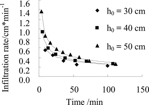
Table 1. Descriptive statistics of soil water content before (θ₀) and after (θ_s) infiltration, Δθ = θ_s – θ₀.

	Min	Max	Mean	Variance	Coefficient of variation	Skewness	Kurtosis
θ0	0.216	0.368	0.278	0.034	0.001	0.532	3.221
θs	0.348	0.432	0.392	0.021	0.001	0.452	3.024
Δθ	0.015	0.147	0.053	0.034	0.001	0.954	3.178

Table 2. The relationship between soil water content change Δθ and the average values of soil saturated hydraulic conductivity k_s and Green-Ampt wetting front suction ψ.

Δθ	h0 = 30 cm		h0 = 40 cm		h0 = 50 cm
	ks /cm*min^−1	ψ/m	ks /cm*min^−1	ψ/m	ks /cm*min^−1	ψ/m
0.01	0.106	0.09	0.102	0.092	0.071	0.085
0.05	0.104	0.093	0.1	0.096	0.069	0.089
0.10	0.099	0.101	0.096	0.103	0.066	0.093
0.15	0.094	0.107	0.092	0.108	0.064	0.097
0.20	0.092	0.112	0.09	0.112	0.063	0.1

Figure 2. The relationships between the parameter values of Ks (A) and Ψ (B) estimated using Δθ measured at every test point and the ones predicted using mean Δθ.

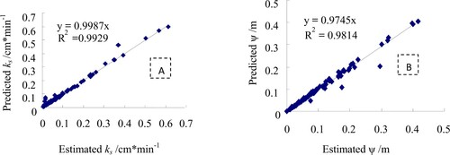
Figure 3. The relationship between estimated soil saturated hydraulic conductivity k_s and infiltration time t_i. CI means cumulative infiltration.

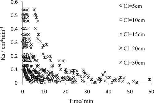
Table 3. Linear regression coefficients between soil saturated hydraulic conductivity k_s and the reciprocal of infiltration time 1/t_i.

Infiltration time /min	h0 = 30 cm	h0 = 40 cm	h0 = 50 cm
t5	0.9261	0.8878	0.7226
t10	0.9894	0.9869	0.906
t15	0.9933	0.9484	0.9614
t20	0.9850	0.9938	0.9808
t25	–	0.9902	0.9933
t30	0.9579	0.9903	0.9664
t35	–	–	0.9405
t40	–	0.9313	0.9208
t50	–	–	0.8733

 –, not available.

Figure 4. The relationship between estimated and predicted values of soil saturated hydraulic conductivity k_s.

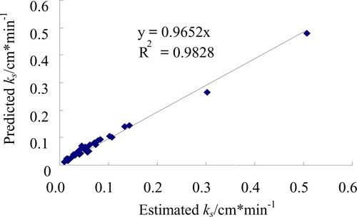
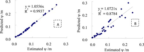
Figure 5. The relationship between estimated Green-Ampt wetting front suction ψ and the ratio of maximum to medium infiltration time t_med/t_max when the initial head height h₀ is constant (A) or variable (B).

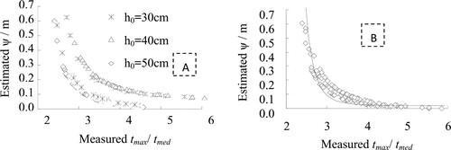
Figure 6. The relationship between estimated and predicted values of Green-Ampt wetting front suction ψ when initial head height h₀ is constant (A) and variable (B).