
Figures & data
Figure 1. An overview map of the study area with locations of the farms investigated in the cropping years 2019–2020 and 2020–2021.
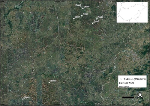
Figure 2. Distribution patterns of mean annual precipitation and mean annual temperature for the period of 2002–2022. Both precipitation and temperature come from aggregated hourly data. Source: Hungarian Meteorological Service.
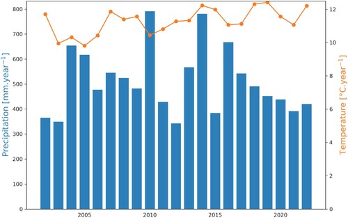
Figure 3. A Bayesian generalised linear model architecture used for our explanatory analysis. The model included five climate variables: The growing degree days (GDD), maximum temperature (Tmax), average temperature (Tavg), minimum temperature (Tmin), and precipitation (Rain). The sigma represents the error term of the model. As all explanatory variables showed a normal distribution, we set the parameters of the prior regression model to ‘Normal’. In this model, the sweet corn yield and GDD were response variables.
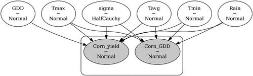
Figure 4. Crop production and financial data (Mean ± sd, N = 5) for the investigated fields for the cropping year periods of 2019–2020 and 2020–2021. (a) Comparison of barley and sweet corn yield between double and single cropping for the 5 farms investigated in this study. Kruskal–Wallis was conducted on double and single cropping systems separately. The letter ‘x’ indicates no significant differences based on bootstrap (10,000 iterations, p < 0.05), (b) Barley and sweet corn yield (combined data) during the cropping years 2019–2020 and 2020–2021 for double and single cropping system, (c) comparison of the benefit–cost ratio between double and single cropping system for the cropping years 2020 and 2021. For all panels, different letters indicate statistically significant differences in the distribution of values based on Kruskal–Wallis and Bootstrap (10,000 iterations, p < 0.05).
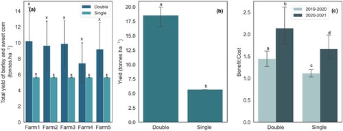
Figure 5. Pearson correlation analysis between variables used in our analysis. (a) the correlation between corn growing days and time (years), (b) the correlation between sweet corn GDD and time, (c) the correlation between barley GDD and time, and (d) the correlation between barley yield and time.
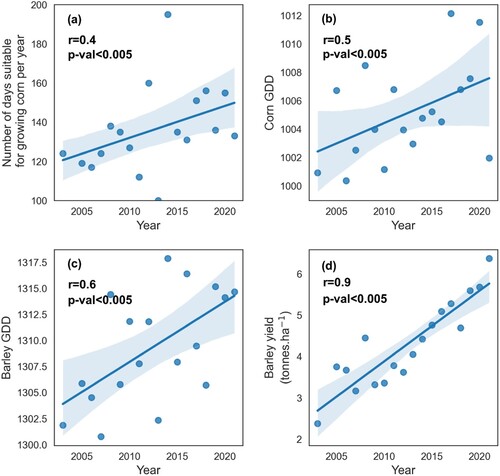
Figure 6. The distribution of standardised posterior effect size of major climatic parameters on (a) sweet corn yield, (b) GDD associated with sweet corn. (Rain) indicates mean annual precipitation, (Tmin) indicates annual minimum temperature, Tavg indicates mean annual temperature, (Tmax) indicates annual maximum temperature, and (GDD) growing degree days. The vertical, dashed line separates negative and positive effects. The white dot indicates the average effect size and the whisker represents a 95% confidence interval.
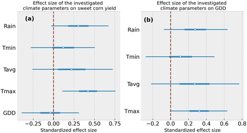
Table 1. Field management practices for the investigated fields.
Figure A1. Model check: a trace plot showing the output of a Markov Chain Monte Carlo (MCMC) sampling process and sampled values of model parameters over the course of the 3000 sampling iterations, and the 6 chains. The left side of the trace plot shows the distribution of parameter values and each horizontal line corresponds to a different parameter (Rain, Tmin, Tavg, Tmax, and GDD) being sampled. The X-axis on the right side shows the iteration of the MCMC sampling process. It shows how the convergence of the parameter values changes over the course of the 3000 sampling iterations. Note the stability of the parameter values throughout the sampling process suggesting that they did not change significantly.
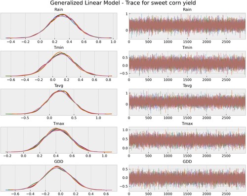
Figure A2. Model check: a trace plot showing the output of the MCMC sampling process and sampled values of model parameters throughout the 3000 sampling iterations, and the 6 chains. The left side of the trace plot shows the posterior distribution of parameter values while the right side shows the convergence of the posterior distribution of the parameter values throughout 3000 iterations and 6 chains. For details see (Figure A1).
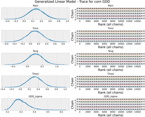
Figure A3. The energy plot shows the marginal energy and the energy transition for the 3000 iterations of the MCMC sampling process. The distribution of the marginal energy values shows the current fit of the model to the data, while the energy transition reveals the progression of the energy values over the course of the sampling process. In this case, the good agreement between the two density plots and the similarity of the two distributions indicates that the model converged and fit well the data at each step of the sampling process.
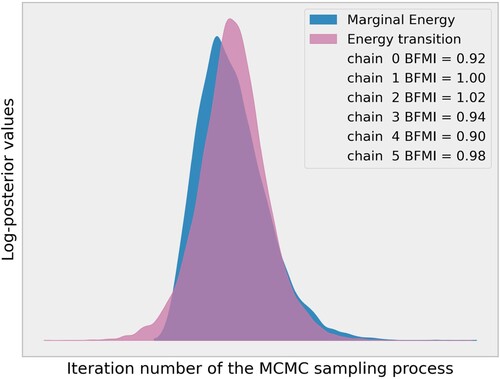
Figure A4. Distribution of major soil properties for the investigated fields. (a) Distribution of soil organic matter content across the investigated fields, (b) Distribution of soil pH, (c) distribution of plant available phosphorus and (d) distribution of plant available potassium. The white dot in the middle indicates the mean value. Note that the Y-axis was rescaled to improve visualisation.
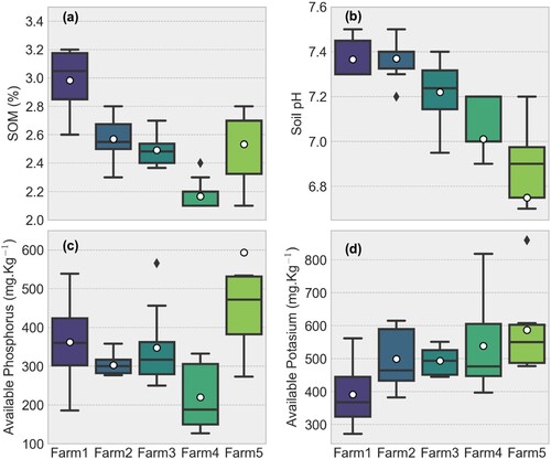
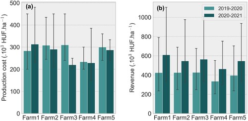
Figure A5. (a) Total production cost and (b) revenue (Mean ± CI, 95%) per farm for the two cropping years investigated in this study. The values are presented in thousands Hungarian forints per hectare.
Data availability statement
All data used to make conclusions in this study are available upon reasonable request to the corresponding author.