Comparative metabolomics of Japanese Black cattle beef and other meats using gas chromatography–mass spectrometry

Figures & data

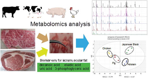
Figure 1. Evaluation of GC/MS for analysis of meat metabolites.

(a) Chromatogram shows the total ion content of muscle tissues isolated from livestock. These chromatographs show a comparison among Japanese black cattle, Holstein, pig, and chickens. Asterisk indicates the peak of IS (16.5 minutes). (b) Venn diagram showing the number of overlapping metabolites with reproducibility between livestock species.

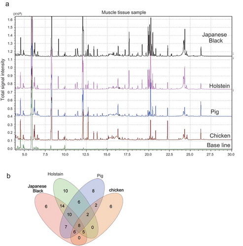
Figure 2. Comparison of detected metabolites between meats.

(a) Scatter plot shows the mean peak intensity of metabolites as indicated by GC/MS (each type of livestock, n = 3). The R² values indicate the degree of correlation. Numbers in A and C indicate the following compounds: 1, mannose; 2, phospholic acid; 3, fructose 1-phosphate; 4, allose; 5, lactic acid; 6, urea; 7, glycine; 8, inositol. (b) PCA score plot demonstrating the correlation in metabolites between livestock species (Scaling, Pareto variance). The PCA model was analyzed using fitting parameters (Components, 4; R² [cum] = 0.960; Q² [cum] = 0.868). (c) The loading plot demonstrates the relationship between metabolite attributes and the PCA plot.

Figure 3. Metabolites that differ significantly between Japanese Black cattle and other livestock.

Fold changes in graphed data indicate significant differences in metabolites (n = 3; p < 0.05). (a) Japanese Black vs. Holstein cattle. (b) Japanese Black cattle vs. pigs. (c) Japanese Black cattle vs. chickens. The data represent the relative values of the normalized peak intensity of meats compared with that of Japanese Black cattle. *significant difference (p < 0.01)

Figure 4. Comparison of metabolite levels between muscle and fat tissue.

(a) Photograph showing the collection of small samples of muscle tissue from marbled beef. (b) To confirm the purity of isolated tissues, tissue-specific marker proteins were detected with immunoblotting. Several pieces of the muscle tissue and intramuscular fat were collected from the center of steak-cut beef. The intermuscular fat was collected from the peripheral area of the steak. (c) OPLS-DA score plot demonstrates the relationship between metabolites in muscle and fat tissue (each tissue type, n = 4; Scaling, Pareto variance). The OPLS-DA model was analyzed using fitting parameters (Components, [1 + 2]; R² [cum] = 0.996; Q² [cum] = 0.987). (d) S-plot of OPLS-DA demonstrates the correlation in metabolites between tissue types. Positive p-values (0 to 1.0) indicate a greater abundance of the metabolite in fat than in muscle; negative p-values (0 to −1.0) indicate a greater abundance of the metabolite in muscle than in fat. (e) The graph demonstrates (mean ± standard error, n = 4) represent the values of metabolites in each tissue.

Figure 5. Comparison of metabolites in different cattle breeds using GC/MS.

(a) OPLS-DA score plot visualizes the relationship between metabolites in Japanese Black and Holstein cattle. Types A and B are genetically different Japanese Black cattle (each type of cattle, n = 6; Scaling, Pareto variance). The OPLS-DA model was used for analysis with fitting parameters (Components, [1 + 2]; R² [cum] = 0.940; Q² [cum] = 0.838). (b) S-plots of OPLS-DA data demonstrating the relationship between metabolites in different cattle breeds. Positive p-values (0 to 1.0) indicate a greater abundance of the metabolite in Holstein than in Japanese Black cattle; negative p-values (0 to −1.0) indicate a greater abundance of the metabolite in Japanese Black than in Holstein cattle. The P [1] axis indicates the metabolites responsible for the difference in score plots. Color gradation in the plots indicates the metabolite classes. (c) Presence of decanoic acid as determined by GC/MS. The signal intensity of decanoic acid was significantly greater in Japanese Black than in Holstein cattle.

Figure 6. Relationships between metabolites and sensory evaluation.

(a) The graph demonstrates the values of flavor intensity in each cattle. For the sensory evaluation, the same sample of the Japanese Black type A, type B and Holstein cattle in Figure 5 were used. (mean ± standard error, each type of cattle, n = 6). (b) O2PLS score plot visualizes the relationship between Japanese Black type A, type B and Holstein cattle using data of metabolites for X variable and result of the sensory evaluation for Y variable (each type of cattle, n = 6; Scaling, UV). The O2PLS model was used for analysis with fitting parameters (Components, [1 + 2]; R2 [cum] = 0.825; Q2 [cum] = 0.967). (c) The loading plot demonstrates the relationship between metabolite and items of sensory evaluation.

Tian H, Lam SM, Shui G. Metabolomics, a powerful tool for agricultural research. Int J Mol Sci. 2016 Nov 17;17;17(11):1871. . PubMed PMID: 27869667; PubMed Central PMCID: PMCPMC5133871.

 Web of Science ®Google Scholar