Figures & data
Figure 1 Schematic drawing of a corrugated transition with a smoothly varying depth. The depth of the corrugation starts from λ/2 at an input radius of ain and decreases gradually to λ/4 at a final radius of aout.
Figure 2 Axisymmetric corrugated λ/2 to λ/4 TE11 to HE11 transition profile for a wave propagating in the z direction. The input at z = 0 is fed by a TE11 mode. The number of slots of corrugation, Nslot, varies between (a) 15, (b) 5, and (c) 3. The input radius is 0.113 cm.
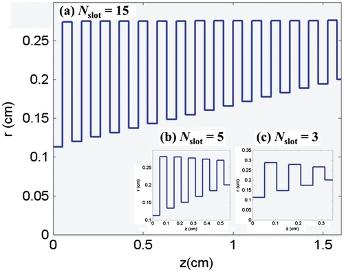
Figure 3 Electric field intensity plots for Nslot = 15 at varying points. The measurements are taken on the xy plane for various values of z. (a) Initially launched waveguide mode at the input port in the TE11 mode, (b) z = 0.23 cm after 2nd slot, (c) z = 0.44 cm after 4 slots, (d) z = 0.97 cm after 9th slot, (e) z = 1.6 cm after 15th slot, and (f) z = 1.7 cm, at which point the beam propagates out of the waveguide.
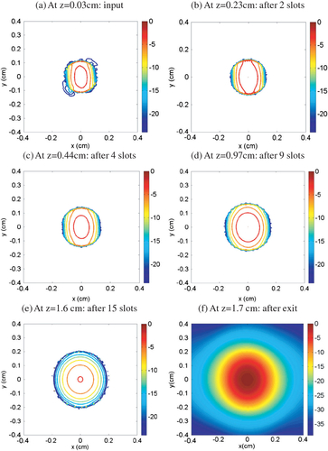
Figure 4 Electric field intensity plots for Nslot = 5 at different values of z measured on the xy plane. (a) Initially launched waveguide mode at the input port (TE11 mode), (b) z = 0.12 cm after 1st slot, (c) z = 0.35 cm after 3rd slot, and (d) z = 0.54 cm after 5th slot.
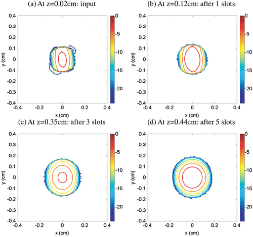
Figure 5 Electric field intensity plots for the Nslot = 3 case at various values of z measured on the xy plane. (a) Initially launched waveguide mode at the input port (TE11 mode), (b) z = 0.13 cm after 1st slot, (c) z = 0.24 cm after 2nd slot, and (d) z = 0.35 cm after 3rd slot.
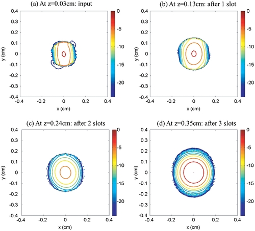
Figure 6 Electric field intensity plotted for the Nslot = 2 case at various values of z measured on the xy plane. (a) Initially launched waveguide mode at the input port (TE11 mode), (b) z = 0.12 cm after 1st slot, (c) z = 0.23 cm after 2nd slot, and (d) z = 0.28 cm where the beam propagates out of the waveguide.
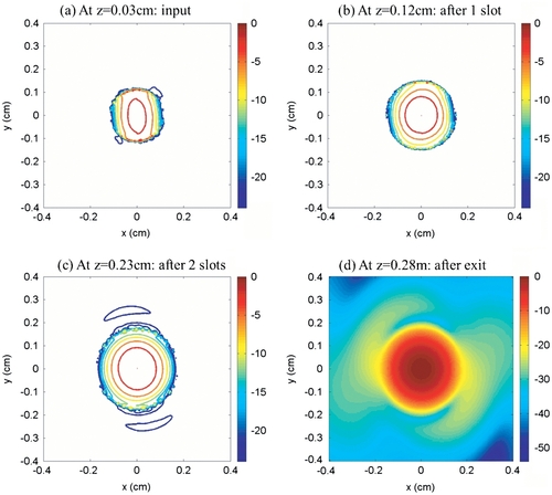
Figure 7 Fabricated corrugated λ/2 to λ/4 mode converters and oversized λ/4 corrugated tapered transitions: (a) λ/2 to λ/4 mode converters with Nslot = 2, 5 and 15, (b), (c), and (d) corrugated λ/4 tapered transitions with Nslot = 2, 5, and 15, respectively with tapered angles of 3° (left) and 10° (right).
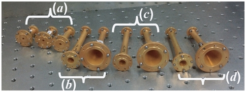
Figure 8 Simulated (a) and experimentally measured (b) return loss with a varying number of corrugation slots (Nslot). The blue circle, black cross, and red dotted curves represent Nslot = 2, 5, and 15, respectively. The cyan triangle represents simulation of Nslot = 3.
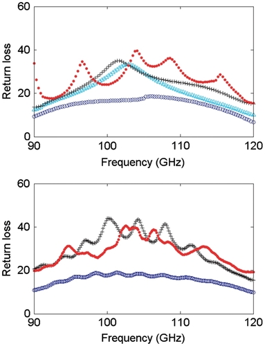
Figure 9 Geometry of a λ/2 to λ/4 transition (TE11 to HE11 mode converter) followed by a λ/4 corrugated tapered section with a taper angle of (a) 10° and (b) 3°. In this geometry, Nslot = 3 in the λ/2 to λ/4 transition.
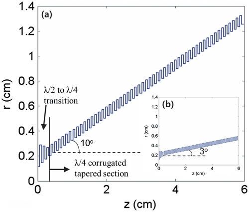
Figure 10 Return loss results of TE11 to HE11 transition as the number of corrugations in the E11 to HE11 transition varies with the attachment of the corrugated tapered section of a depth of λ/4 and varying angle. The simulation results ((a), (b), and (c)) are compared with the experimental results ((d), (e), and (f)). The number of slots (Nslot) is (a), (d): 2, (b), (e): 5, and (c), (f): 15. The black cross and red diamond represent the λ/4 corrugated tapered section with an angle of 3° and 10°, respectively, while the blue open circle represents the case without attachment of the λ/4 corrugated section.
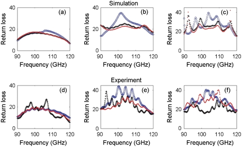
Figure 11 Return loss results for attached λ/4 corrugated tapered transition angles of (a), (c): 3○ and (b), (d): 10○. The simulation results ((a), (b)) are compared with the experimental results ((c), (d)). The blue open circle, black star, and red open triangle represent the number of slots (Nslot) equaling 2, 5, and 15, respectively.
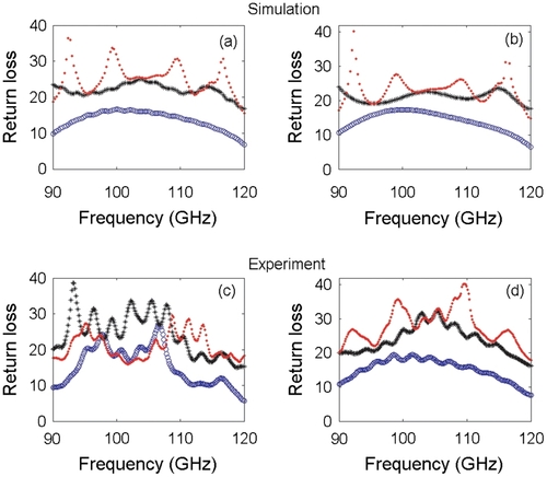
Table 1. Simulation mode contents of λ/2 to λ/4 transition with 3° corrugated tapered transition attached. The λ/2 to λ/4 transition by itself is expressed as “w/o,” while the transition attached to a 3° corrugated tapered transition is expressed as “3°.” The ideal HE11 mode composition is shown in the second row for comparison. All numbers in the table are expressed as percentages.
Figure 12 Electric field intensity and phase plots for HE11 mode input to a λ/4 corrugated transition (Case 1). (a) Electric field intensity plot of cross-polarization (upper plot) and co-polarization (bottom;); (b) unwrapped phase plot of co-polarization electric field cut by x and y axes at the maximum electric field (x,y) location z = 5.1 cm; (c) electric field intensity plot showing cross-polarization (upper plot) and co-polarization (bottom); and (d) unwrapped phase plot of co-polarization electric field cut by x and y axes at maximum electric field (x,y) z = 7 cm.
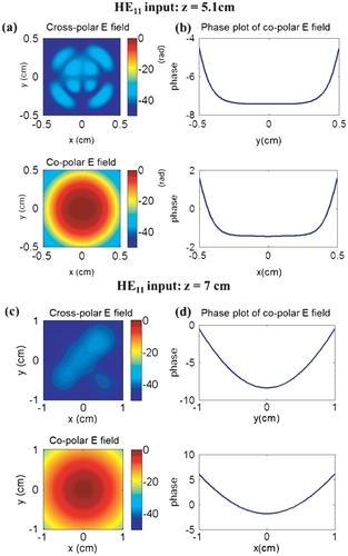
Figure 13 Electric field intensity and phase plots for the TE11 mode input directly to the λ/4 corrugated transition (Case 2). (a) Electric field intensity plot of cross-polarization (upper plot) and co-polarization (bottom;); (b) unwrapped phase plot of co-polarization electric field cut by x and y axes at the maximum electric field (x,y) location z = 5.1 cm; (c) electric field intensity plot showing cross-polarization (upper plot) and co-polarization (bottom); and (d) unwrapped phase plot of co-polarization electric field cut by x and y axes at maximum electric field (x,y) z = 7 cm.
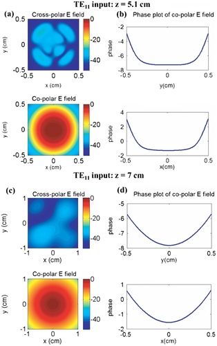
Figure 14 The experimental setup for the field measurement for the 5-cm-long λ/4 corrugated oversized transition without λ/2 to λ/4 transition. The 5-cm-long transition is connected to the one WR-08 frequency extender (TX) and the open waveguide probe is connected to the other WR-08 extender (RCV) to scan the field. The programmable xyz automatic motion controller is mounted on the optical table for the field measurement.
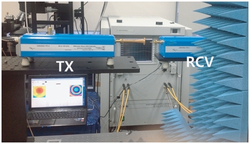
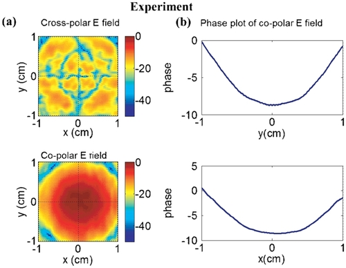
Figure 15 Measured electric field intensity and phase plots for TE11 mode input to the λ/4 corrugated transition (Case 2). (a) Electric field intensity plot of cross-polarization (upper plot) and co-polarization (bottom); (b) unwrapped phase plot of co-polarization electric field cut by x and y axes at maximum electric field (x, y) z = 7 cm.