Electromagnetic analysis and simulation aspects of wireless power transfer in the domain of inductive power transmission technology

Figures & data

Figure 1. IPT charging system for electric vehicle EV.

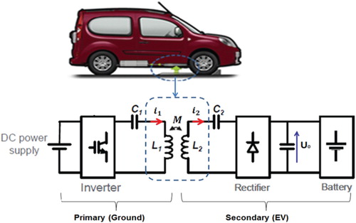
Figure 2. Typical coils for inductive power system (a) circular type (b) rectangular type.

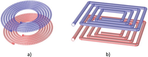
Figure 3. Rectangular system covered by shield [26].

Figure 4. Finite element mesh of a typical circular inductive power system and computed distribution of magnetic flux density vectors (cut plane).

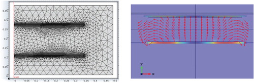
Figure 5. 3D structure with shielding, chassis and measurement positions (stars) for the magnetic field measures.

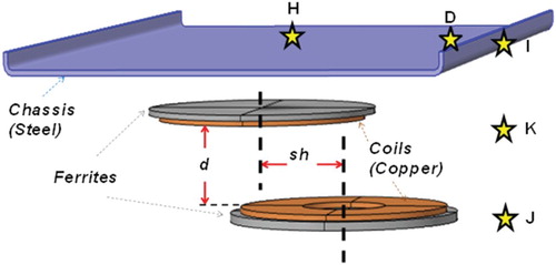
Figure 6. Values of L₁, L₂, M and k due to variation of air gap d(m) for sh = 0 and 0.1 m.

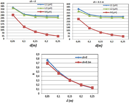
Figure 7. Experimental validation with a chassis of Renault KANGOO.

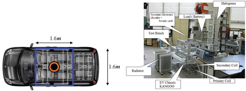
Table 1. Magnitude of the magnetic induction.

Parameter	Measured	Simulated
Point H	0.601 µT	0.002 µT
Point D	1.932 µT	1.876 µT
Point I	4.130 µT	4.800 µT
Point K	4.840 µT	5.010 µT
Point J	4.690 µT	4.650 µT

Figure 8. Parameters of the WPT structure with simple EV chassis.

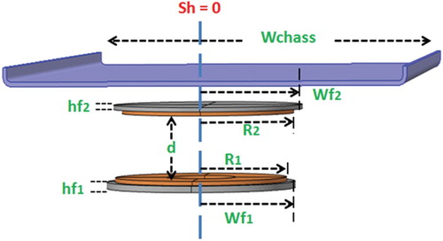
Figure 9. Plot of k in function of the parameterized norm $\frac{R1}{R2}$.

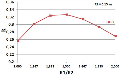
Figure 10. Interoperability prototypes: (a) RNO-NTC (b) NTC-RNO (c) SE-NTC and (d) SE-RNO.

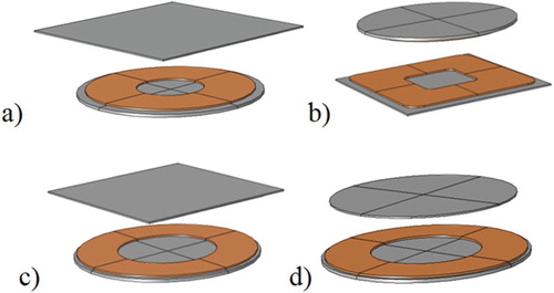
Table 2. Power pad specifications.

Power Pad	Type	Specifications
RNO		Coil	20 Turns
			Copper width 150 mm
			External Diameter 500 mm
		Ferrite	External Diameter 550 mm
SE		Coil	18 Turns
			Copper width 135 mm
			External Diameter 600 mm
		Ferrite	External Diameter 620 mm
NTC		Coil	20 Turns
			Copper width 150 mm
			External width 500 mm
		Ferrite	External width 550 mm

Figure 11. Values of $L_1$ for different prototypes as a function of the air gap distance d(m): (a) sh = 0 and (b) sh = 0.1 m.

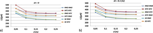
Figure 12. Values of $L_2$ for different prototypes in function of air gap distance d(m): (a) sh = 0 and (b) sh = 0.1 m.

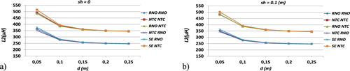
Figure 13. Values of $\text{M}$ for different prototypes in function of air gap distance d(m): (a) sh = 0, (b) sh = 0.1 m.

Figure 14. Values of $k$ for different prototypes in function of air gap distance d(m): (a) sh = 0 and (b) sh = 0.1 m.

Figure 15. Comparison of relative difference of the coupling factor for two groups of reference prototype: (a) $k_{\text{ref}}$: RNO-RNO and (b) $k_{\text{ref}}$: NTC-NTC.

Figure 16. Comparison of values of $|B|$ levels of interoperability prototypes (a) simulation results normalized to test ones and (b) tests results normalized to 6.25 µT.

Table 3. $|B|$ level values for different prototypes.

		SE-RNO		NTC-RNO		NTC-NTC		SE-NTC
		Sim.	Measu.	Sim.	Measu.	Sim.	Measu.	Sim.	Measu.
	H	0.2 µT	0.6 µT	0.2 µT	0.46 µT	0.2 µT	0.3 µT	0.2 µT	0.3 µT
	D	2 µT	2.2 µT	1.4 µT	0.82 µT	4.5 µT	3.65 µT	4.35 µT	3.4 µT
P O I N T	I	4 µT	3.7 µT	3.8 µT	2.5 µT	3.5 µT	2.49 µT	3.3 µT	2.3 µT
	K	5.35 µT	5 µT	5 µT	3.7 µT	8.5 µT	7.08 µT	8.5 µT	7 µT
	J	4.3 µT	4.5 µT	4 µT	3.05 µT	4 µT	3.04 µT	4 µT	3 µT

Figure 17. Human body model and representative wireless inductive charging system.

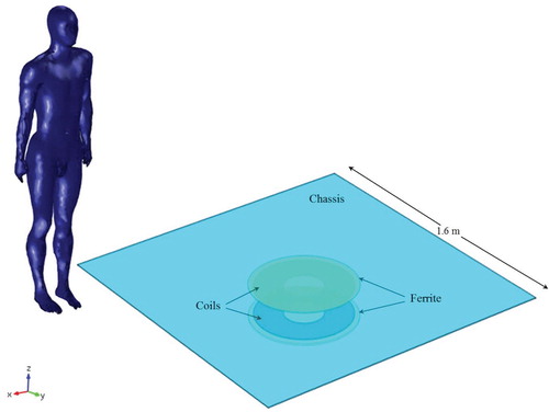
Figure 18. Distribution of induced EMFs inside the human body for the studied configuration. (a) Normalized magnetic flux density B (T); (b) normalized E-field (V/m).

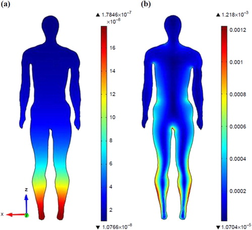
Figure 19. Region of electromagnetic field evaluation.

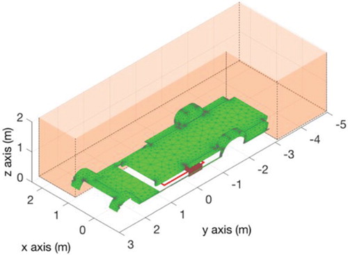
Figure 20. Boundary of the volumes having magnetic flux density higher than the reference level of 27 µT and position of the Duke model for the exposure assessment (blue: receiver on the rear, red: receiver on the center).

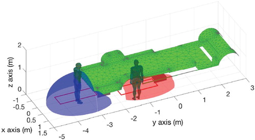
Figure 21. Exposure index on the selected tissues for the analyzed worst cases.

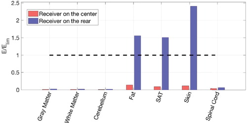
Figure 22. Definition of the safety area. Different volumes where the limit of B is exceeded in blue. Transmitters in red. The dashed one represents the subsequent not active transmitter. The dashed green line represents the border of the safety area.

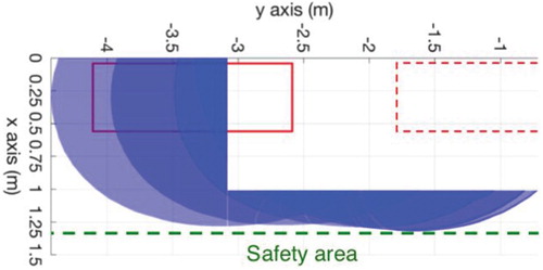
Figure 23. Studied configuration of the WPT system.

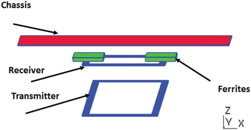
Table 4. Geometrical dimensions.

	Width (m)	Length (m)
Transmitter	0.5	1.5
Receiver	0.5	0.3
Ferrite	0.2	0.25
Frame	1.5	0.5

Table 5. Parameters: range of variations.

	8 points	10 points	15 points
LOO	2.2 × 10^−3	1. × 10^−6	8.1 × 10^−7

Figure 24. Finite element mesh used for computing sampling data.

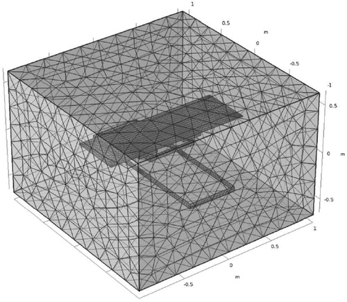
Figure 25. IPT system.

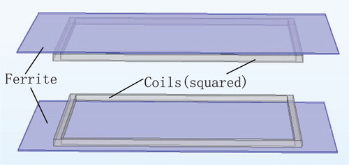
Table 6. LOO values for different numbers of samples.

Parameter	Min	Max
σ (S/m)	10^4	10^6
d (m)	0.	1.
L (m)	0.2	0.3

Table 7. Dimensions of the IPT system.

Parameter	Dimension
Coil length	468 mm
Coil height	13 mm
Ferrite width	600 mm
Ferrite length	500 mm
Ferrite height	2 mm
Distance between coils	150 mm

Figure 26. log (LOO) error versus different number of samples.

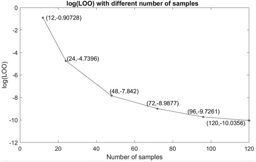
Table 8. Parameters: range of variation.

Parameter	Min	Max
${\mu }_r$	1000	3000
d (mm)	0	15
w (mm)	0	2

Figure 27. First Sobol index versus number of samples.

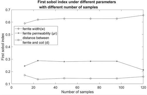
Table 9. Prediction on the mutual inductance.

Samples (w, µr, d)	M (FEM)	M (PCE)	Relative error
(1, 2000, 0.05)	9.33e−6	9.28e−6	0.0058
(1.5, 1500, 0.15)	5.91e−6	5.92e−6	0.0018
(2, 1500, 0.1)	8.04e−6	8.07e−6	0.0035
(2., 2500, 0.05)	9.94e−6	9.81e−6	0.0131
(1,1000,0)	9.33e−6	9.50e−6	0.0181

Figure 28. 3D mesh of the light passenger vehicle.

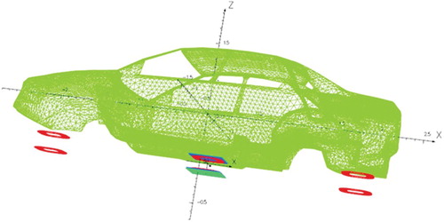
Table 10. Range of variation of the two parameters.

Parameter	Min	Max
${\mu }_r$	1	300
σ (S/m)	10	10^7

Table 11. LOO and Sobol’s indices.

Number of samples	LOO	Sµ	Sσ
16	1.3 × 10^−4	0	0.99
10	2.2 × 10^−3	0	0.99
8	1.2 × 10^−2	2.2 × 10^−4	0.99
5	0.36	5.3 × 10^−3	0.98

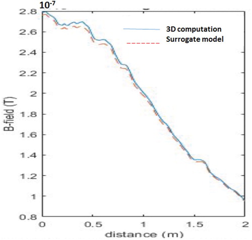
Figure 29. B-field on a vertical line located at 1.5 m from the side of the vehicle.

Mohammad M, Tezera Wodajo E, Choi S, et al. Modeling and design of passive shield to limit EMF emission and to minimize shield loss in unipolar wireless charging system for EV. IEEE Trans Power Electron. 2019;34(12):12235–12245.

 Web of Science ®Google Scholar