Drone-mounted UWB snow radar: technical improvements and field results

Figures & data

Figure 1. Penetration depth at a temperature of 268 K shown as a function of frequency for dry snow with 0.5 mm grain size, wet snow with dry snow density of 0.4 g/ccm, freshwater ice, and impure ice. Dry snow penetration depth is calculated with two different models, where the main difference is that the Tsang model accounts for grain size.

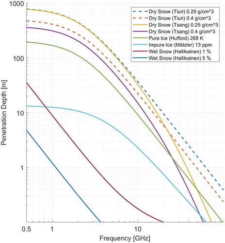
Figure 2. Block diagrams of the UWiBaSS.

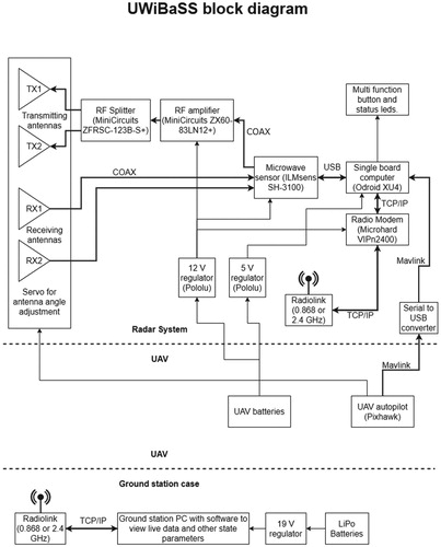
Table 1. UWiBaSS key characteristics.

Attribute	Value
Signal generation	UWB Pseudo noise
System bandwidth	3.8 GHz (0.7–4.5)
Range resolution	≈5 cm
m-sequence clock frequency	13.312 GHz
Measurement rate	52 Hz (max 1000 Hz)
MLBS order	9 (511 range bins)
Nominal output power	17.3 dBm
Unambiguous range in air	5.9 m
Average power consumption	8.1–9 W
Total Weight	≈3 kg
Transmitter
No high voltage peaks
Low field strength operation
Power splitter into Dual Vivaldi antenna prototype
Receiver
Continuous, synchronous sub-sampling operation
Timebase jitter less than 20 fs (rms)
Dual Vivaldi prototype with each antenna
Element into separate channel

Figure 3. Close up of Vivaldi antenna (a), radar system with dual Vivaldi antennas (b), and the same radar system mounted under a UAV (c). (a) Close-up of modified Vivaldi antenna, with resistive loads (1), inserted slits (2) and printed lens in aperture (3). (b) Dual Vivaldi antennas mounted in bistatic configuration (painted black) and (c) Antenna prototype (and radar box) mounted under “Cryocopter FOX”. The antenna angle regulation mechanism have a slight angle when not powered up, to keep tension on stabilizing bungees when pointing in nadir.

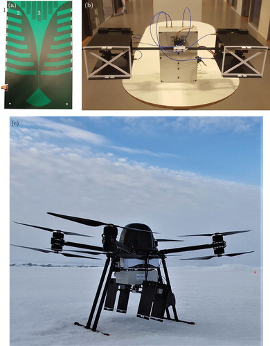
Figure 4. Simulated antenna parameters.

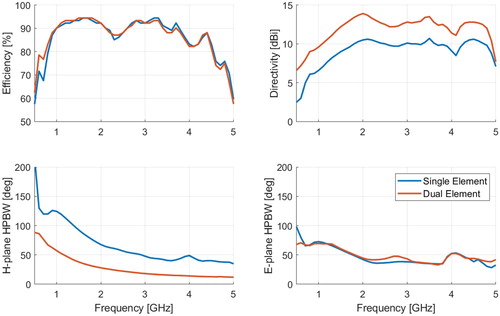
Figure 5. Simulated and measured return loss for the modified Vivaldi antenna.

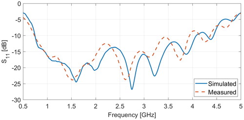
Table 2. Comparison of single Vivaldi antenna and dual modified Vivaldi antenna.

Antenna configuration	Single	Dual with slits
Bandwidth	0.95–6 GHz	0.7–4.5 GHz
Penetration depth^a	9.7 m	18.2 m
Theoretical range resolution	2.97 cm	3.94 cm
Directivity at 2 GHz	10.5 dBi	13.9 dBi

^aCalculated at lowest frequency in bandwidth for snow with 1% liquid water content (LWC).

Figure 6. Example radar image before and after altitude correction.

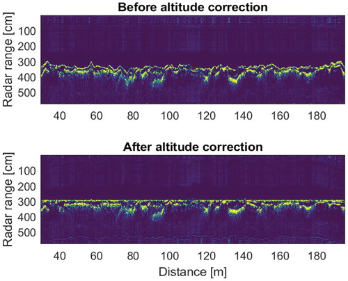
Figure 7. Example showing radar image and UAV altitude with the UAV mostly flying outside the unambiguous range, and entering the ambiguous range at approximately 150 s.

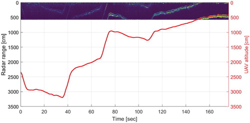
Figure 8. Returned power compared to the theoretical returned power according to the radar equation. Data was collected with a drone-mounted radar with a max unambiguous range of 5.7 m.

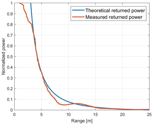
Figure 9. The same data as in Figure 7, before any correction (top) after altitude dependent power calibration (middle) and finally after the shifting procedure (bottom).

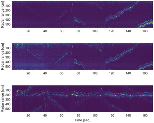
Table 3. Ambiguity windows.

Window number	Start of window	End of window
1	0 m	5.7 m
2	5.7 m	11.4 m
3	11.4 m	17.1 m

Figure 10. Pixel variance of the un-calibrated (top) and range calibrated (bottom) radar image. Ambiguity windows are marked with red diamonds.

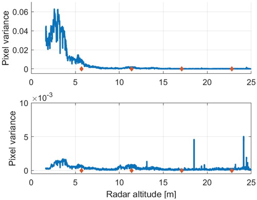
Figure 11. Chart of preferred zones of altitude given different target lengths. This is calculated for a radar system with 5.75 m unambigous range.

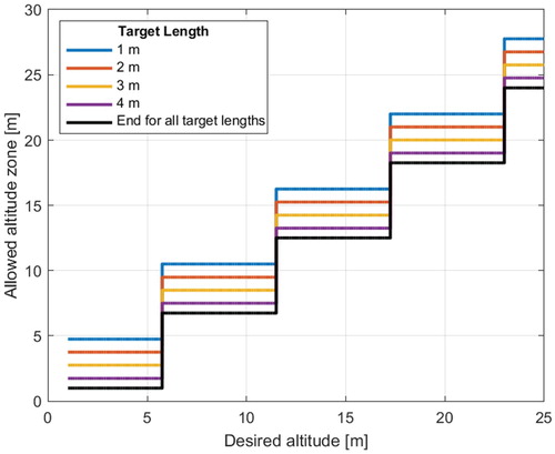
Figure 12. Map of SIOS field locations. Sites visited on the current campaign is marked in red.

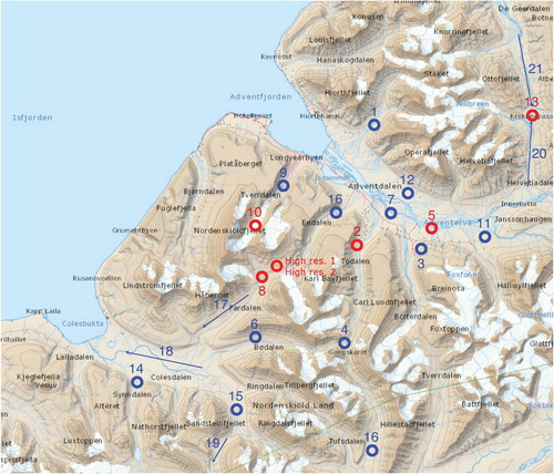
Figure 13. B-scan radar image from site “High res. 1”, with interpreted radar snow depth compared with in situ snow depth. The radar measurement is a 100 m transect with 38 manual measurements over nearly 80 m. All data points are geo-referenced.

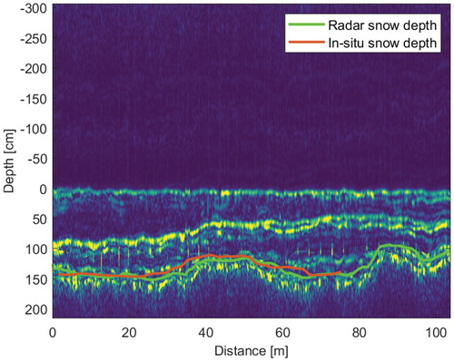
Figure 14. A-scan radar responses in red (150 slow time averages), compared to in situ stratigraphy in blue, assessed using the “hand test” [43] shown with the top x-axis. (a) Site 4 and (b) Site 8.

Figure 15. Georeferenced snow depth from site 2, measured with drone mounted radar (a) and GPS snow probe (b). $C=0.67\pm 0.01$ and root-mean-square error (RMSE) $=5.9$ cm. (a) Radar snow depth and (b) In situ snow depth.

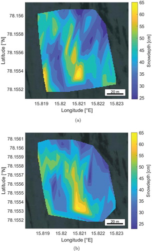
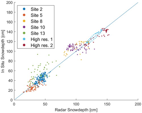
Figure 16. In-situ snow depth vs. radar snow depth for all sites. Spatial correlation: $C=0.97\pm 0.01$ and RMSE $=10.6$ cm.

Greene E, Birkeland K, Elder K. Observation guidelines for avalanche programs in the United States. Bozeman (MT): American Avalanche Association; 2016.

 Google Scholar