Adjustments in the Labor and Real Estate Markets: Estimates of the Time Series Variation in the Natural Vacancy Rate

Figures & data

Table 1. Summary statistics.

	18 MSAs; 1980–2018					61 MSAs; 1990–2018
	Obs.	Mean	SD	Min	Max	Obs.	Mean	SD	Min	Max
Panel (A): annual
Vacancy rate %	702	14.7	5.3	1	31	1769	14.2	4.5	1.4	29.9
Real rent psf per annum	702	32.2	10.3	15.7	83.2	1769	26.9	9.3	13.5	98.8
Office stock (sq. ft. m)	702	92	63	8.1	313.4	1769	58.2	73.6	4	496.6
Office employment (000 s)	702	416	254	52	1145	1769	276	271	32	1869
Vacancy change	684	0.2	2.6	–6.1	15.3	1708	–0.2	2.2	–7.2	14.9
Real rental growth %	684	–0.5	8	–27.6	47.5	1708	–0.4	7.3	–39	56.6
Stock growth %	684	3.5	4.9	0	35.1	1708	1.7	2	–3.8	16.3
Employment growth %	684	2.6	3.6	–14.7	14.2	1708	2	3.6	–17.4	17.6
Panel (B): quarterly
Vacancy rate %	2754	14.9	5.3	1	31.2	6893	14.3	4.5	0.7	30.1
Real rent psf per annum	2754	32.1	10.2	15.7	85.8	6893	26.9	9.3	13.5	98.8
Office stock (sq. ft. m)	2754	92.2	62.8	8.1	313.4	6893	58.2	73.6	4	496.6
Office employment (000 s)	2754	417	253	52	1145	6893	276	271	32	1869
Vacancy change	2736	0.1	1	–7	9.7	6832	–0.1	0.9	–5.1	4.9
Real rental growth %	2736	–0.2	2.7	–15.8	37.7	6832	–0.1	2.5	–17.1	18.8
Stock growth %	2736	0.9	1.4	0	13.3	6832	0.4	0.7	–4.6	7.4
Employment growth %	2736	0.6	1	–5.8	5.6	6832	0.5	1.1	–7.4	6.6

Note. This table reports summary statistics for the variables used in the modeling of vacancy rates and real rents. Panel (A) is for the annual data and Panel (B) is for the quarterly data. The sections on the left are for the longer time series for 18 Metropolitan Statistical Areas (MSAs) for 1980–2018, and those to the right are for the shorter time series for 61 MSAs for 1990–2018. Sample sizes for rates of change are simply number of MSAs multiplied by number of periods (e.g., 18 MSAs x 38 years = 684 observations). However, sample sizes for variables in levels are higher by one more observation per MSA, reflecting that one further set of observations in levels is needed to compute the rate of change for the first period each time (e.g., 684 annual rates of change + 18 further data points = 702 observations).

Figure 1. Changes in aggregate employment, stock, real rent and vacancy rate. Panel A: Office employment and office floorspace over period 1981–2018. Panel B: Real office rent and office vacancy rate over period 1981–2018.

Note. The graphs are based on aggregate series for the sample of 18 MSAs that have data spanning 1981–2018. Employment and stock were summed across the set of markets, while real rent per square foot per annum and vacancy rate were computed as stock-weighted averages of the series for each MSA in the sample.

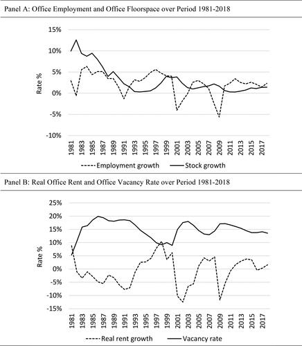
Figure 2. Median vacancy rate and dispersion of vacancy rates across MSAs by year. Panel A: Sample of 18 MSA office markets over period 1980–2018. Panel B: Sample of 61 MSA office markets over period 1990–2018.

Note. The box and whisker plots show the interquartile range (spanned by box) and the full range (from minimum to maximum) in recorded office vacancy rates for that year across the sample of MSAs. The horizontal line inside each box indicates the median vacancy rate in the sample that year.

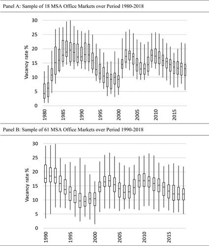
Table 2. Rental change models with a constant NVR.

		Dependent variable: Real rental growth
	Sample	1981–2018	1981Q1–2018Q4	1991–2018	1991Q1–2018Q4
	Variable	Coeff.	Coeff.	Coeff.	Coeff.
Panel (A)	Constant	0.09*	0.03***	0.12*	0.04***
		(2.4)	(4.2)	(2.7)	(5.2)
	Lagged vacancy rate	–0.66**	–0.22***	–0.89**	–0.31***
		(–3.1)	(–5.0)	(–3.3)	(–5.6)
	Adjusted R-squared	17.5%	25.4%	15.1%	25.1%
	Implied NVR	13.6%	14.0%	13.6%	13.7%
Panel (B)	Constant	0.06	0.03**	0.11***	0.04***
		(1.4)	(2.9)	(4.1)	(5.4)
	Lagged vacancy rate	–0.49	–0.18***	–0.81***	–0.29***
		(–1.7)	(–3.3)	(–4.1)	(–5.6)
	Lagged rent error	–0.39***	–0.08**	–0.69***	–0.15***
		(–4.8)	(–3.2)	(–8.0)	(–5.4)
	Adjusted R-squared	48.9%	38.7%	76.0%	54.7%
	Implied NVR	13.2%	13.9%	13.5%	13.7%
Panel (C)	Constant	0.11***	0.03***	0.04	0.02
		(5.0)	(7.2)	(0.8)	(1.8)
	Lagged vacancy rate	–0.84***	–0.23***	–0.50	–0.22**
		(–6.7)	(–9.0)	(–1.5)	(–2.9)
	Lagged rent error	–0.21***	–0.04***	–0.66***	–0.13***
		(–4.2)	(–3.4)	(–4.5)	(–3.8)
	Growth in office employment	1.18***	0.98***	0.35	0.52
		(4.8)	(8.1)	(1.0)	(1.9)
	Growth in office stock	–0.54***	–0.43***	1.32	1.03
		(–4.6)	(–3.8)	(1.2)	(1.1)
	Adjusted R-squared	73.8%	57.5%	77.1%	57.1%
	Implied NVR	12.7%	13.1%	8.5%	10.9%

Note. This table reports the results of the estimation of the rental adjustment model set out in Equation (9)(9) $${rr}_t={\beta }_1\left(v_{t-1}-\mathit{NVR}\right)+{\beta }_2{\mathit{rerr}}_{t-1}+{\beta }_3{d}_t+{\beta }_4{s}_t$$(9) .

$${rr}_t={\beta }_1\left(v_{t-1}-\mathit{NVR}\right)+{\beta }_2{\mathit{rerr}}_{t-1}+d_t+s_t$$

where $\mathit{rerr}$ is the residual from the long run model set out in Equation (8)(8) $$\mathit{ln}{RR}_t^{\mathrm{*}}={\lambda }_0+{\lambda }_1\mathit{ln}{D}_t+{\lambda }_{2}ln\left(S_t\right(1-\mathit{NVR}\left)\right)$$(8) .

$$\mathit{ln}{RR}_t^{}={\lambda }_0+{\lambda }_1\mathit{ln}{D}_t+{\lambda }_{2}ln(S_t(1-\mathit{NVR}))$$

In panel (A), only the lagged vacancy rate is used as a regressor; in panel (B), the lagged rent error is added; and in panel (C), the shock variables, growth in office employment and the growth in stock, are added. The dependent variable is the difference in the natural log of the level of real rent, which approximates the rate of growth in real rents. The models are estimated using annual and quarterly data and for 1981–2018 and 1991–2018. These specifications assume that the natural vacancy rate (NVR) is constant in time. All estimations use HAC standard errors and covariances (Bartlett kernel, Newey-West fixed bandwidth = 5.0). The reported test statistics are from t-tests and (^*) indicates significance at 5%; (^**) indicates significance at 1%; and (^***) indicates significance at 0.1%.

Figure 3. Estimates of the natural vacancy rate from the short run rent model using rolling 10-year windows. Panel A: Sample of 18 MSAs for windows ending 1990–2018, annual LHS and quarterly RHS. Panel B: Sample of 61 MSAs for windows ending 2000–2018, annual LHS and quarterly RHS.

Note. Model A is the traditional rental adjustment model shown in Equation (6)(6) $${rr}_t={\beta }_1\left(v_{t-1}-\mathit{NVR}\right)$$(6) . Model B adds the residual error from Equation (7)(7) $${rr}_t={\beta }_1\left(v_{t-1}-\mathit{NVR}\right)+{\beta }_2{\mathit{rerr}}_{t-1}$$(7) to the specification of Model A. While we also estimated Equation (8)(8) $$\mathit{ln}{RR}_t^{\mathrm{*}}={\lambda }_0+{\lambda }_1\mathit{ln}{D}_t+{\lambda }_{2}ln\left(S_t\right(1-\mathit{NVR}\left)\right)$$(8) , a short run rent model that includes shock variables, estimates of the natural vacancy rate based on this are unstable so are not shown. In each case, the NVR is estimated from the regression coefficients as –β₀/β₁.

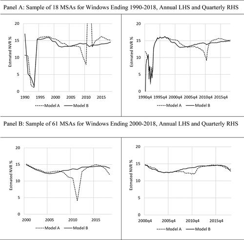
Table 3. Cross-section variation in the NVR from the short run ECM models.

	1981–2018		1981Q1–2018Q4		1991–2018		1991Q1–2018Q4
	Mean and standard deviation
Panel (A)	Mean	SD	Mean	SD	Mean	SD	Mean	SD
Model A	12.5%	2.3%	13.4%	2.3%	12.0%	4.0%	12.7%	3.2%
Model B	13.5%	2.3%	13.9%	2.4%	12.6%	3.2%	12.9%	3.0%
Model C	10.7%	2.1%	12.6%	2.2%	11.3%	2.7%	12.1%	2.8%
Panel (B)	Correlations between models
	Model A	Model B	Model A	Model B	Model A	Model B	Model A	Model B
Model B	93.2%		99.1%		97.7%		99.6%
Model C	85.1%	88.5%	97.8%	98.3%	88.7%	93.0%	98.2%	98.9%
Panel (C)	Correlations with actual average
Model A	77.6%		91.3%		60.9%		73.4%
Model B	95.0%		96.0%		75.9%		79.2%
Model C	82.7%		93.4%		82.3%		81.1%

Note. This table presents summary statistics for the NVR estimates from panel versions, with MSA and time fixed effects, of the three real rental growth models presented in Table 2. Model (A) includes only the lagged vacancy rate; model (B) adds the lagged rent error; and model (C) adds the shocks variables – growth in office employment and growth in stock. The models are estimated using annual and quarterly data and for 1981–2018 and 1991–2018. For each model, the mean and standard deviation of the cross-section estimates of the MSA natural vacancy rates are presented and, below these, are the correlations among the models. The means and standard deviations are given in percentages. The correlations with the actual averages are for the time series averages for each MSA.

Figure 4. Estimates of the natural vacancy rate based on time fixed effects in a short run rent model, annual data. Panel A: Sample of 18 MSA office markets over period 1980–2018. Panel B: Sample of 61 MSA office markets over period 1990–2018.

Note. Model A is the traditional rental adjustment model shown in Equation (6)(6) $${rr}_t={\beta }_1\left(v_{t-1}-\mathit{NVR}\right)$$(6) . Model B adds the residual error from Equation (7)(7) $${rr}_t={\beta }_1\left(v_{t-1}-\mathit{NVR}\right)+{\beta }_2{\mathit{rerr}}_{t-1}$$(7) to the specification of Model A. Model C adds shock variables and is shown in Equation (8)(8) $$\mathit{ln}{RR}_t^{\mathrm{*}}={\lambda }_0+{\lambda }_1\mathit{ln}{D}_t+{\lambda }_{2}ln\left(S_t\right(1-\mathit{NVR}\left)\right)$$(8) . All three models include time and MSA fixed effects. The results from estimation of these models on quarterly frequency data show the same general pattern. Because they are much noisier, they are not shown.

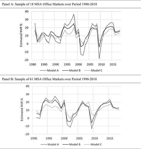
Table 4. Estimates of the NVR from persistence models for whole US.

		1981–2018	1981Q1–2018Q4	1991–2018	1991Q1–2018Q4
Voith and Crone	NVR	15.6%	16.3%	13.0%	11.8%
	Persistence	0.76	0.96	0.80	0.98
Marston (m = 3)	NVR	15.3%	15.9%	13.5%	12.9%
	Persistence	0.44	0.94	0.33	0.95
Grenadier	NVR	16.3%	68.9%	25.1%	24.1%
	Persistence	0.72	0.98	0.63	0.95

Note. This table presents the results of three types of persistence models used to estimate the NVR, from Marston (1985), Voith and Crone (1988) and Grenadier (1995). The figures are for estimates of the persistence of a shock to the vacancy rate and the implied NVR. All models are estimated using US level data and so produce a single national estimate of the NVR. The models are estimated using annual and quarterly data and for 1981–2018 and 1991–2018. Without a time-varying NVR, the Voith and Crone annual model is the Marston model with a lag of one year (m = 1). For the quarterly Voith and Crone model, we use a lag of one quarter. For the Marston model, after a three-period lag (m = 3), the persistence estimates are very close to one, so the NVR estimates are very large and are not presented. The NVR estimates are given as percentages.

Table 5. Estimates of the NVR from persistence models using panel models.

	1981–2018		1981Q1–2018Q4		1991–2018		1991Q1–2018Q4
Panel (A): Marston	m = 4	m = 3	m = 4	m = 3	m = 4	m = 3	m = 4	m = 3
Estimates of MSA NVRs
Mean	15.4%	15.6%	15.5%	15.6%	13.5%	13.4%	13.6%	13.5%
SD	2.8%	2.8%	2.7%	2.8%	2.3%	2.3%	2.3%	2.3%
Correlation with quarterly	99.9%	99.9%			99.9%	99.9%
Correlation with actual average	99.2%	99.2%	99.1%	99.2%	97.4%	97.0%	97.5%	97.2%
Persistence
Common	0.70	0.73	0.91	0.92	0.61	0.69	0.88	0.91
Panel (B): Voith & Crone			Persistence
	Com.	MSA	Com.	MSA	Com.	MSA	Com.	MSA
Estimates of MSA NVRs
Mean	15.7%	15.9%	16.1%	16.4%	13.1%	13.0%	12.9%	14.0%
SD	2.9%	2.8%	2.9%	3.2%	2.3%	3.7%	2.3%	7.8%
Correlation with quarterly	99.8%	97.9%			99.5%	–59.3%
Correlation with actual average	98.6%	96.9%	97.7%	92.0%	94.2%	66.6%	91.3%	–7.7%
Persistence
Common	0.78		0.96		0.80		0.96
Mean		0.80		0.96		0.80		0.95
SD		0.06		0.02		0.11		0.03
Panel (C): Grenadier			Persistence
	Com.	MSA	Com.	MSA	Com.	MSA	Com.	MSA
Estimates of MSA NVRs
Mean	22.4%	23.0%	41.7%	28.4%	24.3%	10.0%	21.9%	19.6%
SD	2.9%	3.0%	3.1%	4.1%	2.3%	149.4%	2.3%	59.9%
Correlation with quarterly	99.0%	21.3%			98.8%	8.1%
Correlation with actual average	98.8%	86.0%	95.8%	56.7%	96.1%	–9.4%	91.6%	–25.7%
Persistence
Common	0.77		0.97		0.76		0.96
Mean		0.77		0.97		0.75		0.95
SD		0.04		0.01		0.11		0.03

Note. This table presents the results of the panel versions, with MSA and time fixed effects, of the three types of persistence models used to estimate the NVR, from Marston (1985), Voith and Crone (1988) and Grenadier (1995). The models are estimated using annual and quarterly data and for 1981–2018 and 1991–2018. The results from the all US versions are in Table 4. The figures are for estimates of the persistence of a shock to the vacancy rate and the implied NVR. Without a time-varying NVR, the annual Voith and Crone model is the Marston model with a lag of one year (m = 1 for the annual data). For the quarterly model, we use a lag of one quarter. Marston (1985) used m = 4 and m = 8. As we could not estimate the all US model with m = 4 and presented m = 3, we present m = 3 and m = 4 versions here. The NVR estimates are given as percentages. The correlations with the actual averages are for the time series averages for each MSA.

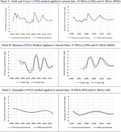
Figure 5. Estimates of time variation in natural vacancy rate using persistence models. Panel A: Voith and Crone’s (1988) method applied to annual data, 18 MSAs (LHS) and 61 MSAs (RHS). Panel B: Marston’s (1985) method applied to annual data, 18 MSAs (LHS) and 61 MSAs (RHS). Panel C: Grenadier’s (1995) method applied to annual data, 18 MSAs RHS and 61 MSAs LHS.

Note. The Voith & Crone specification is shown in Equation (15)(15) $${\epsilon }_{it}={\rho }_i{e}_{it-1}+{\gamma }_t+{\mu }_{it}$$(15) , the Marston specification in Equation (12)(12) $${\epsilon }_{i,t}=\rho {\epsilon }_{i,t-1}+{\eta }_{i,t}$$(12) and the Grenadier specification in Equation (16)(16) $$v_{it}={\alpha }_i\left(1-{\rho }_i\right)+{\gamma }_t+{\rho }_i{v}_{it-1}+{\mu }_{it}$$(16) . The results indicate the percentage point variation from the mean natural vacancy rate for each model shown in Table 5. The use of an MSA persistence term makes little difference from assuming common persistence across the set of markets, so the lines are very similar. Results from estimation of the models on quarterly frequency data show the same general pattern, although they are much noisier, so are not shown.

Marston, S. (1985). Two views of the geographic distribution of unemployment. The Quarterly Journal of Economics, 100(1), 57–79. https://doi.org/https://doi.org/10.2307/1885735

 Web of Science ®Google Scholar

Voith, R., & Crone, T. (1988). National vacancy rates and the persistence of shocks in U.S. office markets. Real Estate Economics, 16(4), 437–458. https://doi.org/https://doi.org/10.1111/1540-6229.00467

 Web of Science ®Google Scholar

Grenadier, S. R. (1995). Local and national determinants of office vacancies. Journal of Urban Economics, 37(1), 57–71. https://doi.org/https://doi.org/10.1006/juec.1995.1004

 Web of Science ®Google Scholar