Theory and practice of higher-order frequency modulation synthesis

Figures & data

Figure 1. Flowcharts for PM (left) and FM (right).

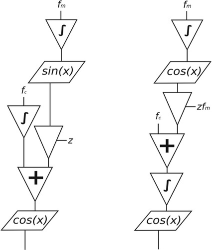
Figure 2. Naïve second-order FM stack.

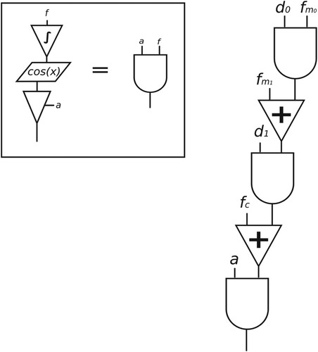
Figure 3. Spectrogram of naïve second-order stacked FM output, with $f_{m_0}=f_{m_1}=f_c=500$ Hz, $d_1=f_{m}0$, applying a linear envelope to $d_0$, $0\le d_0<2f_{m_0}$.

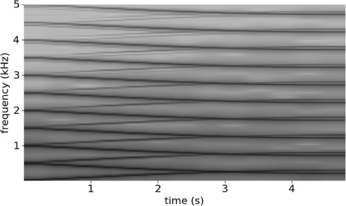
Figure 4. Spectrogram of naïve second-order stacked FM output, with $f_{m_0}=f_{m_1}=f_c=500$ Hz, $d_0=f_{m}0$, applying a linear envelope to $d_1$, $0\le d_1<2f_{m_1}$.

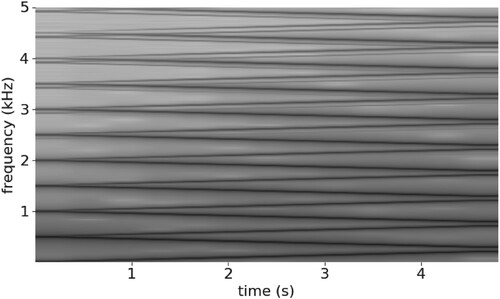
Figure 5. Second-order FM flowchart.

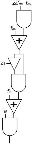
Figure 6. Second-order FM (left) and PM (right) waveforms and normalised spectra from Equation (12(12) $\begin{array}{rl}& m_0(t)=\cos (2\pi f_{m_0}t)\\ & m_1(t)=\cos (2\pi {\int }_0^t{f}_{m_1}+z_0{f}_{m_0}{m}_0(x)\mathrm{d}x)\\ & c(t)=\cos (2\pi {\int }_0^t{f}_c\\ & +z_1[f_{m_1}+z_0{f}_{m_0}{m}_0(x)]m_1(x)\mathrm{d}x\phantom{\int }).\end{array}$(12) ) (Figure 5) and Equation (15(15) $c(t)=\cos (2\pi f_{c}t+z_1\sin (2\pi f_{m_1}t+z_0\sin (2\pi f_{m_0}t))).$(15) ), respectively, with $f_c=f_{m_0}=f_{m_1}=500$ Hz, $z_0=3$, and $z_1=2$.

Figure 7. FM operator (left) and second-order modulation arrangement (right). The a and f parameters represent the scalar index/amplitude and frequency.

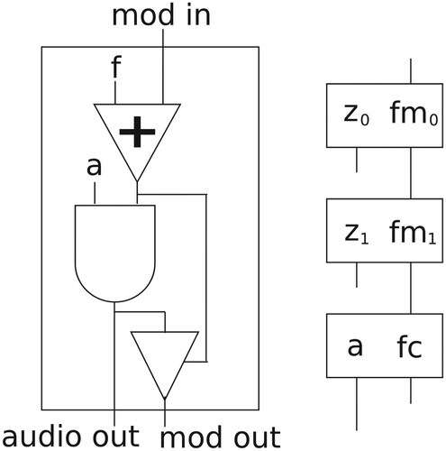
Figure 8. FM operator with feedback (left) and its black-box representation (right).

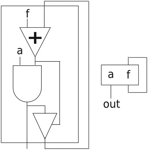
Figure 9. Feedback hoFM (left) and PM (right) waveforms and spectra, with f = 500 Hz.

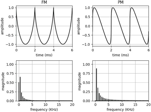
Figure 10. FM operator including an internal feedback path with independent control of amplitude (a) and feedback gain ($|g|\le 1$) (left) and its black-box representation (right).

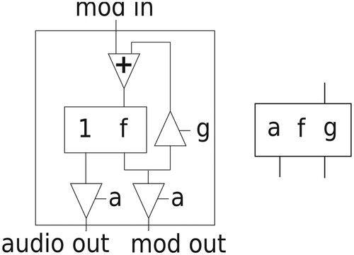
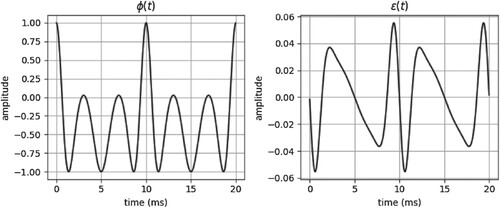
Figure 11. Modulation $\varphi (t)$ (left) and error $ϵ(t)$ (right) from Equation (31(31) $ϵ(t)=\nu (t)-\varphi (t).$(31) ), with $f_{m_0}=f_{m_1}=100$ Hz, $z_0=3$, and $f_s=44.1$ KHz.