Sulphuric precipitates in novel titanium-based, sulphur-bearing bulk metallic glass – a BMG composite?

Figures & data

Figure 1. (a) Synchrotron diffraction data I(Q) for three different plates. The insert displays the BSE contrast SEM images as well as the determined area percentage (A%) of precipitated phases. (b) Synchrotron X-ray diffraction spectra, resulting from the 2 mm thick plate of Ti₄₀Zr₃₅Cu₁₇S₈ (solid blue line), shown together with the theoretical spectrum (in orange), combining amorphous background (blue dashed line) and calculated intensity from the Rietveld refined (Ti, Zr)₂Cu cell, as well as the residual (solid black line).

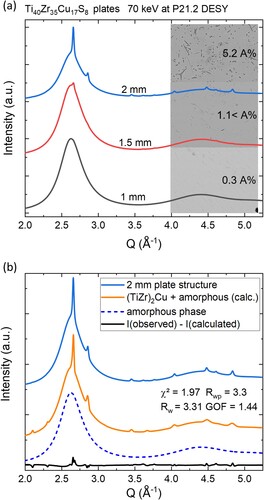
Figure 2. (a) SEM image in BSE contrasting mode showing a precipitate in the synchrotron X-ray amorphous 1.5 mm plate sample. (b) In-lens detector image, showing mainly material contrast of the FIB cut lamella with applied protective Pt-cover applied on top, for later thinning operation. The section of the sample where TEM analysis was performed on this specimen is marked by a dashed rectangle labelled TEM.

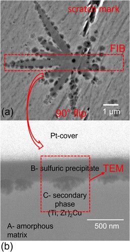
Figure 3. (a) Local TEM-EDS analysis results for the three different phases, namely the local amorphous matrix (A), the sulphuric precipitate (B) and the secondary phase (C) as well as SEM-EDS results of the global matrix phase and the nominal composition for reference. (b) TEM bright-field image of the interface between sulphuric precipitate (B) and local matrix phase (A), containing the secondary phase (C) as well as their diffraction images. The corresponding TEM-EDS spectra are shown in Figure 4.

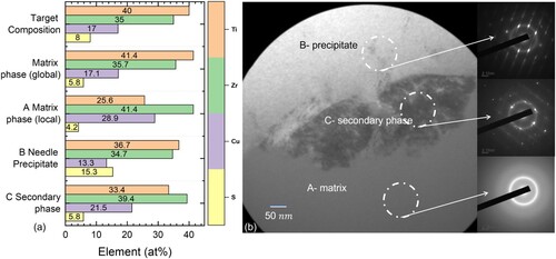
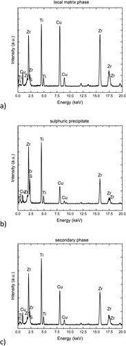
Figure 4. TEM-EDS spectra of (a) the local matrix phase, (b) the sulphuric precipitate and (c) the secondary phase.