2,168
Views
2
CrossRef citations to date
0
Altmetric
Original Articles

Machine configuration and workload balancing of modular placement machines in multi-product PCB assembly

, &
Pages 815-830 | Received 26 Apr 2017, Accepted 05 Jan 2018, Published online: 24 Jan 2018

Figures & data

Figure 1. A gantry-type placement machine with three identical configurable modules. Each module has a single gantry mechanism, multi-nozzle head and a feeder unit.

Figure 1. A gantry-type placement machine with three identical configurable modules. Each module has a single gantry mechanism, multi-nozzle head and a feeder unit.

Table 2. Parameters.

Table 3. Configuration parameters of a sample MCLB-M problem.

Figure 2. Multi-model Evolutionary Algorithm (MEA) for machine module configuration and line balancing.
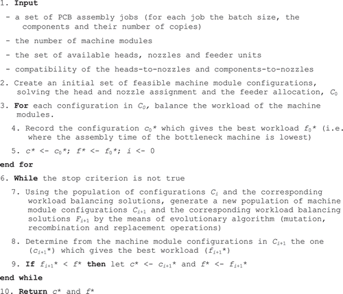
Figure 2. Multi-model Evolutionary Algorithm (MEA) for machine module configuration and line balancing.

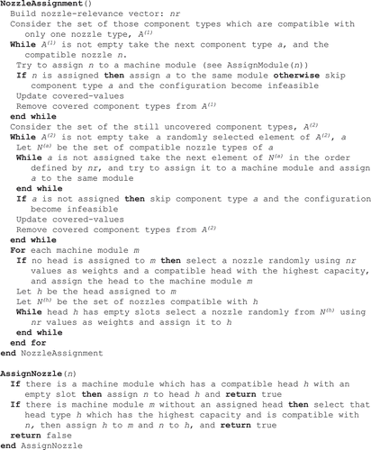
Figure 3. Pseudo code for initial nozzle assignment.

Figure 3. Pseudo code for initial nozzle assignment.

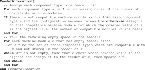
Figure 4. Pseudo code of the feeder allocation.

Figure 4. Pseudo code of the feeder allocation.

Figure 5. Nozzle list (N’) of three machine modules.

Figure 5. Nozzle list (N’) of three machine modules.

Figure 6. A recombination operation on two sample configurations with 3 machine modules, 3 head types (capacities 4, 3, 2) and 6 nozzle types. The Boolean vector for modules is v = (1 1 0) and Boolean vector for nozzles of module 1 is w = (0 1 0 1). In offspring 2, the first head is then sorted by the nozzle identifiers.
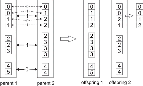
Figure 6. A recombination operation on two sample configurations with 3 machine modules, 3 head types (capacities 4, 3, 2) and 6 nozzle types. The Boolean vector for modules is v = (1 1 0) and Boolean vector for nozzles of module 1 is w = (0 1 0 1). In offspring 2, the first head is then sorted by the nozzle identifiers.

Table 4. Basic parameters of problem instances in single PCB cases.

Table 5. Summary of test results for the problem instances of with traveling times 1 and 10.

Table 6. Parameter values for the generated test instances.

Table 7. Results obtained using MEA in the multi-model case of random generated test instances got by averaging twenty independent runs.

Table 8. The production time of PCB types in different production plans.

Figure 7. The effect of the number of different PCB types on the average production time per PCB type, the average running time of MEA and the average number of generations (where the final solution was first found by MEA). The x-axis gives us the number of PCB types in the production plan. The results are averages of 20 independent runs with all possible PCB type combinations for each number of different types (i.e. one PCB type, two PCB types, etc.).
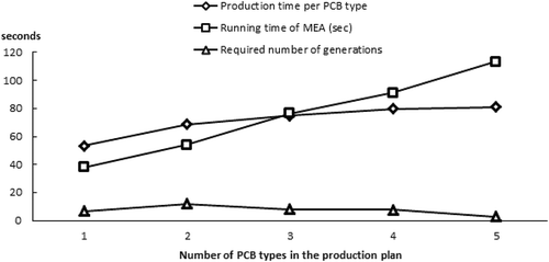
Figure 7. The effect of the number of different PCB types on the average production time per PCB type, the average running time of MEA and the average number of generations (where the final solution was first found by MEA). The x-axis gives us the number of PCB types in the production plan. The results are averages of 20 independent runs with all possible PCB type combinations for each number of different types (i.e. one PCB type, two PCB types, etc.).