Reinforcement learning based optimal decision making towards product lifecycle sustainability

Figures & data

Table 1. Summary of the literature on the decision-making for product lifecycle management.

Reference	Area	Decision process	Key technique	Data source
Zhang et al. (2017b)	Manufacturing industry	Maintenance service stage	Big data analytics	Onsite observations, interviews and reports
Ferreira et al. (2017)	Automotive industry	Planning, machining and evaluation stages	Knowledge-based collaborative processes	Original equipment manufacturers and suppliers
Rondini et al. (2017)	Automotive industry	Maintenance service stage	Discrete event simulation with agent-based modelling	Truck maintenance company
Badurdeen, Aydin, and Brown (2018)	Manufacturing industry	Product design stage	Non-dominated sorting genetic algorithm II	Toner cartridge company
Kaewunruen and Lian (2019)	Infrastructure industry	Planning and design, manufacturing, pre-assembly, logistic, reconstruction and installation, operation and maintenance, demolition and recycle/renewal stages	Digital twin (building Information modelling)	Raw data from the field
Li, Zhong, and Lin (2019)	Aero-engine maintenance	Maintenance service stage	Reinforcement learning	Hypothetical data
Yao et al. (2020)	Infrastructure industry	Maintenance service stage	Deep reinforcement learning	Expressway data
Yousefi, Tsianikas, and Coit (2020)	Dynamic maintenance policy	Maintenance service stage	Reinforcement learning	Hypothetical data
Liu et al. (2020a)	Manufacturing industry	Co-creation, tracking and tracing, maintenance and recycling service stages	Industrial blockchain	Smart gateway by IoT sensors and RFID
Andriotis and Papakonstantinou (2020)	Inspection and maintenance planning	Maintenance service stage	Deep reinforcement learning	Hypothetical data
This paper	Manufacturing industry	Middle of life stage (operation and maintenance) with environmental impacts	Reinforcement learning	Empirical data of the case company with limited availability

Figure 1. AI for product lifecycle management.

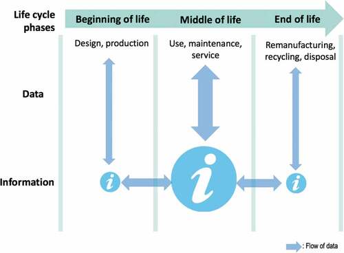
Figure 2. The simplified product lifecycle from a maintenance perspective.

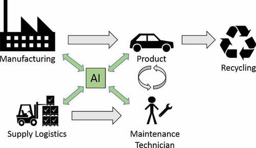
Figure 3. Some RL scenarios.

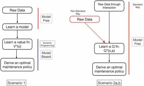
Figure 4. Example 1: Hidden failure rate for Product-X.

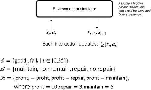
Figure 5. Example 1: the simulation model.

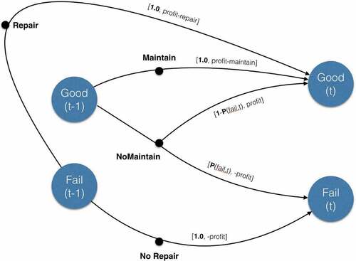
Figure 6. Example 1: optimal policy.

Figure 7. Example 1: maintenance crossover.

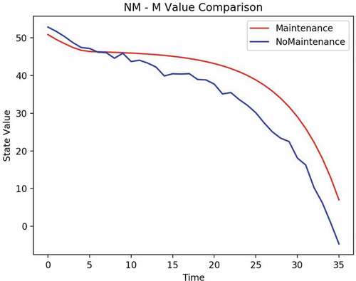
Figure 8. Example 1: reward validation.

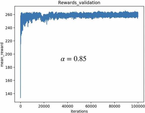
Figure 9. Example 1: mean rewards.

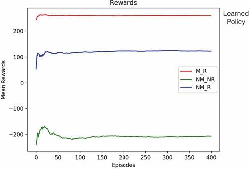
Figure 10. Example 1: MTTF.

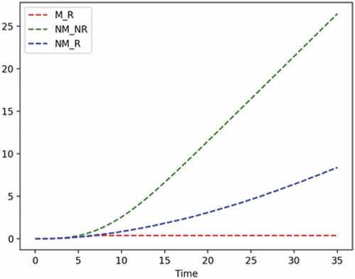
Figure 11. Example 2: hidden failure rate with energy cost.

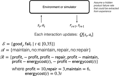
Figure 12. Example 2: the simulation model.

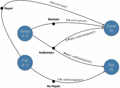
Figure 13. Example 2: optimal policy.

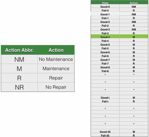
Figure 14. Example 2: maintenance crossover.

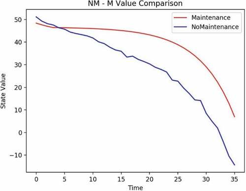
Figure 15. Example 2: reward validation.

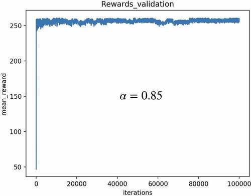
Figure 16. Example 2: mean rewards.

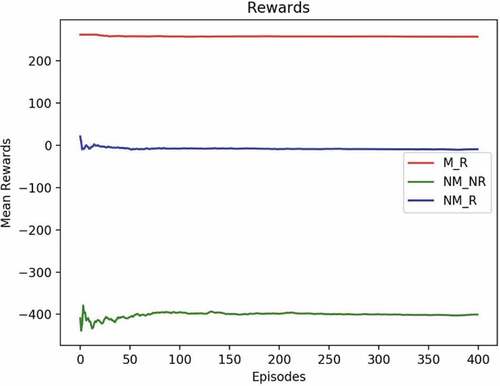
Figure 17. Example 2: MTTF.

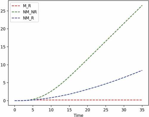
Figure 18. Comparison of learned and simulated failure rate.

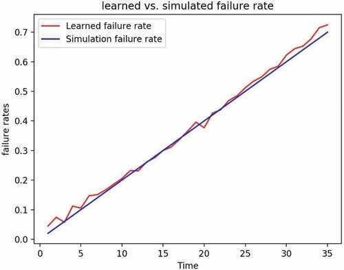
Figure 19. RL extends learning to simultaneously solving a decision problem. Given just a problem state x_t and a reward for that state r_t, the agent will try to learn how to maximise the profits or minimise the costs over time. This can be visualised as a Bayesian network augmented with action nodes, where at each point in time t it has to make a decision based on the history of observed states and rewards.

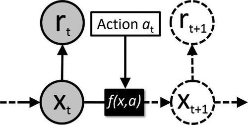
Figure A1. RL overview.

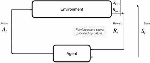
Figure B1. Q-Learning using interaction.

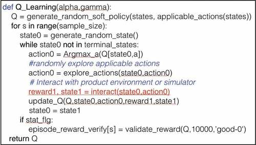
Figure B2. Q-Learning using raw data.

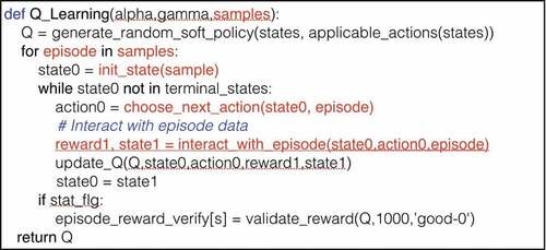
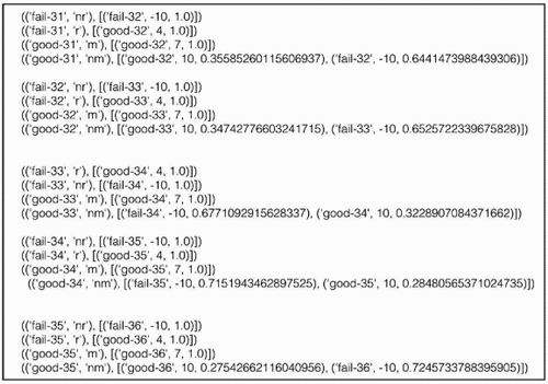
Figure C1. Months 0–9.

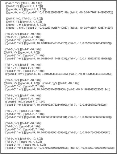
Figure C2. Months 10–19.

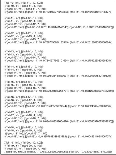
Figure C3. Months 20–29.

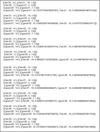
Figure C4. Months 30–35.

Zhang, Y., S. Ren, Y. Liu, and S. Si. January 2017b. “A Big Data Analytics Architecture for Cleaner Manufacturing and Maintenance Processes of Complex Products.” Journal of Cleaner Production 142: 626–641. Elsevier Ltd. 10.1016/j.jclepro.2016.07.123.

 Web of Science ®Google Scholar

Ferreira, F., J. Faria, A. Azevedo, and L. A. Marques. 2017. “Product Lifecycle Management in Knowledge Intensive Collaborative Environments: An Application to Automotive Industry.” International Journal of Information Management 37 (1): 1474–1487. doi:10.1016/j.ijinfomgt.2016.05.006. Elsevier Ltd: 1474–1487.

 Web of Science ®Google Scholar

Rondini, A., F. Tornese, M. G. Gnoni, G. Pezzotta, and R. Pinto. 2017. “Hybrid Simulation Modelling as A Supporting Tool for Sustainable Product Service Systems: A Critical Analysis.” International Journal of Production Research 55 (23): 6932–6945. doi:10.1080/00207543.2017.1330569. Taylor and Francis Ltd.

 Web of Science ®Google Scholar

Badurdeen, F., R. Aydin, and A. Brown. November 2018. “A Multiple Lifecycle-Based Approach to Sustainable Product Configuration Design.” Journal of Cleaner Production 200: 756–769. Elsevier Ltd. 10.1016/j.jclepro.2018.07.317.

 Web of Science ®Google Scholar

Kaewunruen, S., and Q. Lian. August 2019. “Digital Twin Aided Sustainability-Based Lifecycle Management for Railway Turnout Systems.” Journal of Cleaner Production 228: 1537–1551. Elsevier Ltd. 10.1016/j.jclepro.2019.04.156.

 Web of Science ®Google Scholar

Li, Z., S. Zhong, and L. Lin. 2019. “An Aero-Engine Life-Cycle Maintenance Policy Optimization Algorithm: Reinforcement Learning Approach.” Chinese Journal of Aeronautics 32 (9): 2133–2150. doi:10.1016/j.cja.2019.07.003. Chinese Journal of Aeronautics.

 Web of Science ®Google Scholar

Yao, L., Q. Dong, J. Jiang, and F. Ni. 2020. “Deep Reinforcement Learning for Long‐term Pavement Maintenance Planning.” Computer-Aided Civil and Infrastructure Engineering 35 (11): 1230–1245. doi:10.1111/mice.12558. Blackwell Publishing Inc.

 Web of Science ®Google Scholar

Yousefi, N., S. Tsianikas, and D. W. Coit. 2020. “Reinforcement Learning for Dynamic Condition-Based Maintenance of a System with Individually Repairable Components.” Quality Engineering 32 (3): 388–408. doi:10.1080/08982112.2020.1766692. Taylor and Francis Inc.

 Web of Science ®Google Scholar

Liu, X. L., W. M. Wang, H. Guo, A. V. Barenji, Z. Li, and G. Q. Huang. June 2020a. “Industrial Blockchain Based Framework for Product Lifecycle Management in Industry 4.0.” Robotics and Computer-Integrated Manufacturing 63: 101897. Elsevier Ltd: 101897. 10.1016/j.rcim.2019.101897.

 Web of Science ®Google Scholar

Andriotis, C. P., and K. G. Papakonstantinou. 2020. “Deep Reinforcement Learning Driven Inspection and Maintenance Planning under Incomplete Information and Constraints.” ArXiv, July. arXiv. http://arxiv.org/abs/2007.01380.

 Google Scholar