Predictions of in-situ melt pool geometric signatures via machine learning techniques for laser metal deposition

Figures & data

Figure 1. Schematic description of the workflow applied in this study. The training set for the ML algorithms consists of three groups of data: pre-defined process parameters, process signatures extracted from in-situ image data, and target features. The input features were selected based on spearman<apos;>s correlation with target features. Six different ML algorithms were implemented and compared for predictive performance.

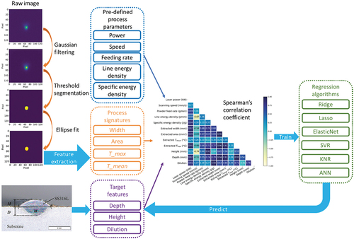
Figure 2. Schematic of the combined experimental apparatus, including laser head, infrared (IR) camera, and laser optics (fibre optic, collimating lens, dichroic mirror, and focusing lens).

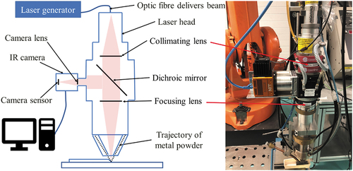
Figure 3. Cross-section of typical single-track deposition (Trial 59). $H$, $D$, and $W$ denote track height, depth, and width, respectively.

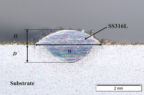
Table 1. Printing parameters used to fabricate all 60 single-track samples. The precisions of the laser power, scanning speed, and powder feed rate was 1 W, 1 mm/s, and 0.1 g/min, respectively

Trial no.	Laser power (kW)	Scanning speed (mm/s)	Powder feed rate (g/min)	Trial no.	Laser power (kW)	Scanning speed (mm/s)	Powder feed rate (g/min)
1	1	10	15.8	31	2.5	20	24.9
2	1	20	15.8	32	2.5	30	24.9
3	1	30	15.8	33	2.5	40	24.9
4	1	10	18.8	34	2.5	20	27.9
5	1	20	18.8	35	2.5	30	27.9
6	1	30	18.8	36	2.5	40	27.9
7	1	10	21.8	37	2.5	20	30.9
8	1	20	21.8	38	2.5	30	30.9
9	1	30	21.8	39	2.5	40	30.9
10	1.5	20	18.8	40	3	20	24.9
11	1.5	30	18.8	41	3	30	24.9
12	1.5	40	18.8	42	3	40	24.9
13	1.5	20	21.8	43	3	20	27.9
14	1.5	30	21.8	44	3	30	27.9
15	1.5	40	21.8	45	3	40	27.9
16	1.5	20	24.9	46	3	20	30.9
17	1.5	30	24.9	47	3	30	30.9
18	1.5	40	24.9	48	3	40	30.9
19	2	30	18.8	49	1.5	10	18.8
20	2	40	18.8	50	1.5	10	21.8
21	2	50	18.8	51	1.5	10	24.9
22	2	30	21.8	52	2.5	20	21.8
23	2	40	21.8	53	2.5	30	21.8
24	2	50	21.8	54	2.5	40	21.8
25	2	30	24.9	55	3	20	21.8
26	2	40	24.9	56	3	30	21.8
27	2	50	24.9	57	3	40	21.8
28	2	20	18.8	58	3	20	33.9
29	2	20	21.8	59	3	30	33.9
30	2	20	24.9	60	3	40	33.9

Figure 4. Row width distribution from the threshold segmentation image shown in Table 2, column 3, trial 58.

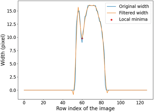
Table 2. Three typical raw melt pool images and their subsequent processing steps

Trial no.	Raw image	Gaussian filtering	Threshold segmentation	Ellipse fit
10
55
58

Figure 5. (a) Comparison between the track width measured via an optical microscope and the melt pool width after all the image processing steps described in section 2.3. The (b) absolute errors between two widths.

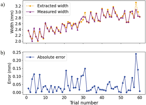
Table 3. Error evaluations between track width measured via an optical microscope and the melt pool width after all the image processing steps described in section 2.3. The precisions of MAE and MXAE are $\pm$ 1 µm

MAE (mm)	MXAE (mm)	MAPE (%)	MXAPE (%)
0.043	0.240	1.8	8.3

Figure 6. Spearman<apos;>s rank correlation coefficient map for each variable pairing from the predefined process parameters extracted melt pool features and measured track geometries.

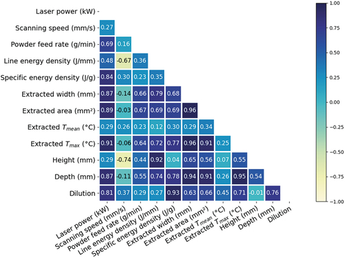
Table 4. Input and output variables for all machine learning models tested here

Lasso, Ridge, ElasticNet, SVR, KNR		ANN characteristics
Inputs	Output	Inputs	Outputs
$LP$, $LED$, $SED$, $W$, $A$, $T_{max}$	$D$	$LP$, $SS$, $LED$, $SED$, $W$, $A$, $T_{max}$	$D$, $H$, $Di$
$SS$, $LED$, $W$	$H$	$LP$, $SS$, $FR$, $LED$, $SED$, $W$, $A$, $T_{max}$, $T_{mean}$	$D$, $H$, $Di$
$LP$, $SED$, $W$, $A$, $T_{max}$	$Di$

Table 5. Hyperparameter candidates for different supervised machine learning algorithms used in this research

Algorithms	Hyperparameter	Description	Candidates
Ridge	$\lambda$	L2 regularisation parameter	10^–3, 10^–2, 10^–1, 1, 10
Lasso	$\lambda$	L1 regularisation parameter	10^–3, 10^–2, 10^–1, 1, 10
ElasticNet	$\lambda$	L2 regularisation parameter	10^–3, 10^–2, 10^–1, 1, 10
	$\alpha$	The ratio of L2 `	0.25, 0.5, 0.75
SVR	$K\left(x\right)$	Kernel functions	polynomial, RBF, sigmoid
	$C=\frac{1}{2\lambda }$	L2 regularisation parameter	10^–3, 10^–2, 10^–1, 1, 10
	$d$	Degree of the polynomial kernel	2, 3
KNR	$k$	Number of neighbours	3, 4, 5, 6, 7
ANN	$\lambda$	L2 regularisation parameter	10^–3, 10^–2, 10^–1, 1
	$n_{neuron}$	Neuron number	1, 2, …, 2 n +3 (n = inputs)
	$n_{layer}$	Hidden layer number	1, 2
	$\phi \left(x\right)$	Activation function	Relu, Logistic
		Learning rate mode	Adaptive, Constant

Table 6. Optimised hyperparameter for all machine learning models tested here

Models	Depth	Height	Dilution
Lasso	$\lambda$=10^−3	$\lambda$=10^−2	$\lambda$=10^−3
Ridge	$\lambda$=10^−3	$\lambda$=10^−1	$\lambda$ =10^−3
ElasticNet	$\lambda$=10^−3, $\alpha$ =0.25	$\lambda$=10^−2,$\alpha$=0.5	$\lambda$=10^−3, $\alpha$ =0.25
SVR	$C$=1, RBF kernel	$C$=10, RBF kernel	$C$=10, RBF kernel
KNR	$k$=6	$k$=7	$k$=4
ANN [7 11 3]	Relu, $\lambda$=10^−3, constant learning rate: 0.01
ANN [7 17 8 3]	Relu, $\lambda$=10^−3, constant learning rate: 0.01
ANN [9 14 3]	Relu, $\lambda$=10^−2, constant learning rate: 0.01
ANN [9 17 9 3]	Relu, $\lambda$=10^−2, constant learning rate: 0.01

Table 7. R² values for all machine learning models tested here. These data characterise how well each regression model fits the observed data (measured melt pool depth, height, and dilution) for each train, CV, and test datasets

Models	Depth			Height			Dilution
	Train	CV	Test	Train	CV	Test	Train	CV	Test
Lasso	0.948	0.921	0.913	0.882	0.809	0.787	0.931	0.910	0.883
Ridge	0.950	0.927	0.910	0.885	0.804	0.761	0.933	0.915	0.882
ElasticNet	0.949	0.925	0.912	0.883	0.809	0.779	0.932	0.913	0.883
SVR	0.973	0.934	0.958	0.940	0.784	0.846	0.976	0.935	0.956
KNR	0.921	0.908	0.937	0.845	0.752	0.734	0.930	0.911	0.904
ANN [7 11 3]	0.983	0.887	0.948	0.972	0.955	0.961	0.968	0.947	0.933
ANN [7 17 8 3]	0.987	0.908	0.953	0.960	0.916	0.947	0.982	0.934	0.938
ANN [9 14 3]	0.990	0.909	0.957	0.978	0.970	0.969	0.976	0.928	0.925
ANN [9 17 9 3]	0.988	0.910	0.958	0.981	0.963	0.948	0.983	0.937	0.947

Table 8. Error measure values when predicting melt pool depth for all machine learning models tested here. The rank assigned to each model is calculated from its mean rank when the models are compared according to their MAE, MXAE, MAPE, and MXAPE values. The precisions of the dimensioned error measures, MAE and MXAE, are both $\pm$ 1 µm

Models	MAE (mm)	MXAE (mm)	MAPE (%)	MXAPE (%)	Rank
Lasso	0.070	0.141	57	343	9
Ridge	0.070	0.140	55	341	7
ElasticNet	0.070	0.140	56	341	7
SVR	0.044	0.132	30	159	4
KNR	0.054	0.119	32	124	3
ANN [7 11 3]	0.049	0.139	34	157	6
ANN [7 17 8 3]	0.039	0.153	18	78	4
ANN [9 14 3]	0.041	0.144	17	44	2
ANN [9 17 9 3]	0.036	0.127	11	30	1

Figure 7. Mean Absolute Error (MAE) and standard deviation for melt pool depth prediction for all machine learning models tested here.

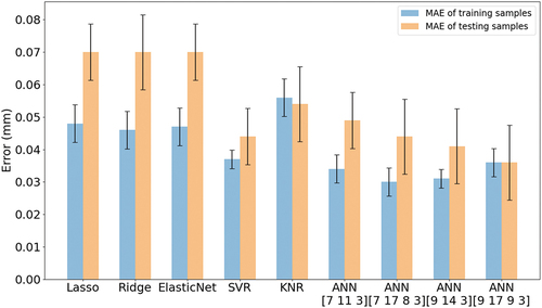
Figure 8. Mean Absolute Error (MAE) and standard deviation for melt pool height prediction for all machine learning models tested here.

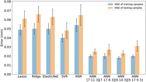
Table 9. Error measure values when predicting melt pool height for all machine learning models tested here. The rank assigned to each model was calculated from its mean rank when the models were compared by their MAE, MXAE, MAPE, and MXAPE values. The precisions of the dimensioned error measures, MAE and MXAE, are $\pm$ 1 µm

Models	MAE (mm)	MXAE (mm)	MAPE (%)	MXAPE (%)	Rank
Lasso	0.061	0.113	16	26	5
Ridge	0.066	0.118	18	27	8
ElasticNet	0.063	0.115	16	27	7
SVR	0.048	0.114	13	30	6
KNR	0.065	0.139	18	52	9
ANN [7 11 3]	0.026	0.054	8	21	2
ANN [7 17 8 3]	0.024	0.077	7	26	3
ANN [9 14 3]	0.023	0.040	7	17	1
ANN [9 17 9 3]	0.030	0.056	8	16	3

Figure 9. Mean Absolute Error (MAE) and standard deviation for melt pool dilution prediction for all machine learning models tested here.

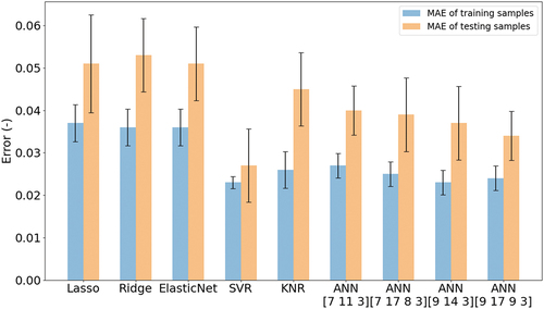
Table 10. Error measure values when predicting melt pool dilution for all machine learning models tested here. The rank assigned to each model is calculated from its mean rank when the models are compared by their MAE, MXAE, MAPE, and MXAPE values

Models	MAE (-)	MXAE (-)	MAPE (%)	MXAPE (%)	Rank
Lasso	0.051	0.104	25	175	7
Ridge	0.053	0.111	24	162	9
ElasticNet	0.051	0.107	25	171	7
SVR	0.027	0.072	8	25	1
KNR	0.045	0.120	20	75	6
ANN [7 11 3]	0.040	0.092	15	58	5
ANN [7 17 8 3]	0.038	0.087	12	41	3
ANN [9 14 3]	0.037	0.105	13	40	4
ANN [9 17 9 3]	0.034	0.078	10	26	2

Table 11. Rank values for predicting melt pool depth, height, and dilution for all the machine learning models tested in this investigation. A smaller average rank indicates the better overall performance of the model

Models	Rank
	Depth	Height	Dilution	Average
Lasso	9	5	7	7.0
Ridge	7	8	9	8.0
ElasticNet	7	7	7	7.0
SVR	4	6	1	3.7
KNR	3	9	6	6.0
ANN [7 11 3]	6	2	5	4.3
ANN [7 17 8 3]	4	3	3	3.3
ANN [9 14 3]	2	1	4	2.3
ANN [9 17 9 3]	1	3	2	2.0

Figure 10. Comparison between the predictions from ANN [9 17 9 3] and measurements from the cross-sections of a single-track build (Trial 40).