Integrated assessment modelling of degrowth scenarios for Australia

Figures & data

Figure 1. An illustrative representation of a possible global mitigation strategy towards net zero emissions that is more commonly modelled (‘Common mitigation modelling’), versus an illustrative scenario that limits activity growth (‘Degrowth logic’), with similar levels of emissions reduction ambition. This is a global aggregate picture, which does not reflect the regional differentiation that is articulated in the degrowth literature, which talks about futures with stronger emissions reductions in the Global North and increases in service provisioning for countries with widespread poverty. Note also that ‘Demand: aggregate services’ (in blue) refers to the aggregated demand for various services, e.g. amount of kilometres travelled, calories eaten or inhabited flat size. This category is most directly affected by avoid-measures in the avoid-shift-improve framework (see Creutzig et al. (2018)).

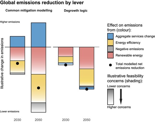
Figure 2. Model interaction flowchart of the MESSAGE-MACRO module tandem.

Black: features common to original and our modified version; red: original version only; blue: modified version only. Slanted boxes contain input and output variables; variables passed on between steps are placed between arrows. Our termination criterion is $Termcrit=\frac{|usefulenergydemand\text{-}exogenoususefulenergydemand|}{exogenoususefulenergydemand}<0.01$.

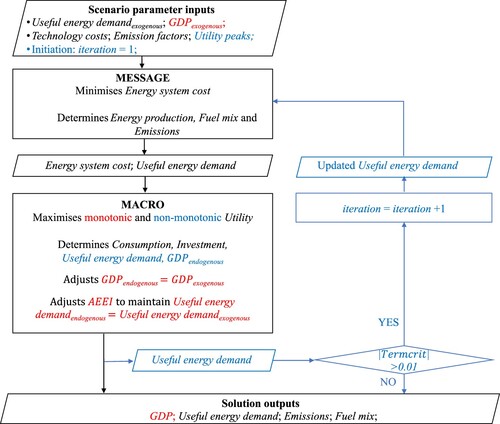
Figure 3. CES function for monotonic ($U$, top) and non-monotonic ($U^{\ast }$, bottom) preferences, in a two-good economy, with ${\alpha }_1=0.55$, ${\alpha }_2=0.45$, and $\sigma =0.05$ (Leontief), $\sigma =1$ (Cobb-Douglas) and $\sigma =10$ (substitutes), and for $U^{\ast }$ with ${\eta }_0=0.15$ and $\xi =-1.5\times {10}^{-3}$. Utility increases from blue to yellow. Contours are asymmetric because of unequal consumption shares.

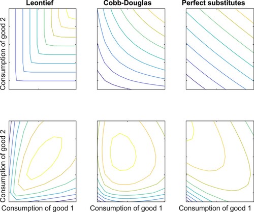
Table 1. Summary of scenario definitions.

Scenarios	Technology cost assumptions	GHG budget	Carbon tax US$/tCO2
Fossil fuel-dominated energy system	Fixing technology costs at historical levels without any future cost variations	N/A	0
Renewable-dominated energy system	Cost reductions of up to 55-90% for wind/solar technologies and 10% for fossil fuels	N/A	0
1.5°C-compliant energy system	Cost reductions of up to 55-90% for wind/solar technologies and 10% for fossil fuels	4 Gt CO2-e from 2020 to 2100	30 (between 2020–2100)

Note that in this study, we focus on trade-offs/interactions between technology-focused levers and degrowth; we, therefore, account for land use, land-use change, and forestry (LULUCF) emissions as a static emission component fixing at 2020 levels (i.e. −39 Mt CO₂-e (Department of Climate Change, 2022)) for all scenarios in all future years:

Figure 4. GDP, physical energy use and GHG emissions under three technology development patterns: a&b, GDP and per-capita GDP for 2020-2100. c&d, total and per-capita physical energy use for 2020-2100. Technology development pattern ranges are indicated by pale-coloured fans. e-j, total and per-capita Australia annual GHG emissions excluding LULUCF for 2020–2100 under three technology development patterns: 1) fossil fuel-dominated energy system (e&f); 2) renewable energy transformation without (g&h) and 3) with (i&j) a large-scale adoption of CCS and NETs. Historial LULUCF emissions are only shown in panels g&h for illustrative purposes; Future LULUCF emissions are assumed to be fixed at 2020 levels (i.e. −39 Mt CO₂-e (Department of Climate Change, 2022)) for all scenarios. Only scenarios i&j are 1.5°C-compliant: emissions budgets are constrained to 4Gt (see Technology development iii in Section 2.3 for scenario definitions). Red lines indicate the SSP2 baseline scenario simulated by the unmodified ‘growth-embedded’ MESSAGE IAM. Colored lines represent ‘growth-decoupled’ scenarios from the modified MESSAGE IAM, assuming consumption utility peaks between 10 - 70 US$k/capita (US$2005). Utility peaks are reached in the year 2100 for SSP2 baseline scenario, and in 2030–2060 for various limited-and de-growth scenarios. UNITS: t US$ = trillion US$; Mt CO₂-e = million tonnes CO₂-e;

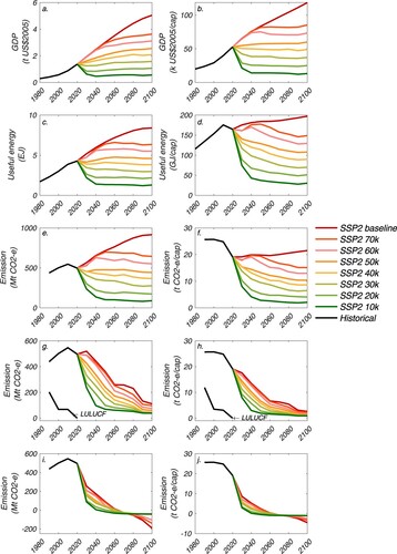
Figure 5. Technology generation mix under three technology development patterns: fossil fuel-dominated energy system (a, corresponding to Figure 4 e&f); renewable energy transformation without (b, corresponding to Figure 4 g&h) and with a large-scale adoption of CCS and NETs (c, corresponding to Figure 4 i&j; 1.5°-compatible); The eight stacked bars in every year set represent the SSP2 baseline scenario (1^st bar; unmodified monotonic MESSAGE) and ‘growth-decoupled’ scenarios assuming consumption utility peaks between 70 - 10 US $k/capita (the 2nd-to-8^th bar), respectively.

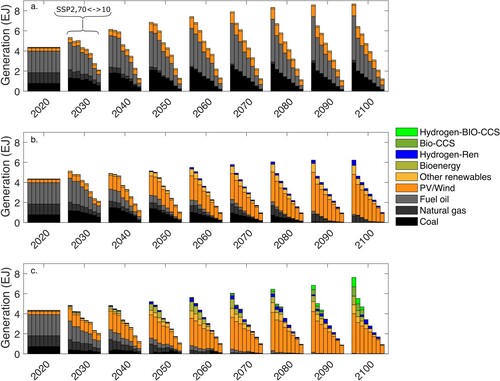
Figure 6. GHG emission reduction levers in the 1.5°-compatible pathways (corresponding to Figure 4 i&j). The eight stacked bars from left to right represent the SSP2 baseline scenario (1st bar; unmodified monotonic MESSAGE) and ‘growth-decoupled’ scenarios with consumption utility peaks between 70 - 10 US $k/capita, respectively. Net GHG reductions: changes in GHG emissions (Figure 5c) w.r.t. the baseline scenario; Demand: GHG emissions level attributable to changes in useful energy; BECCS: Reductions attributable to bioenergy with carbon capture and storage; Bioenergy: Reductions attributable to bioenergy without carbon capture and storage (e.g. biofuels for vehicles).

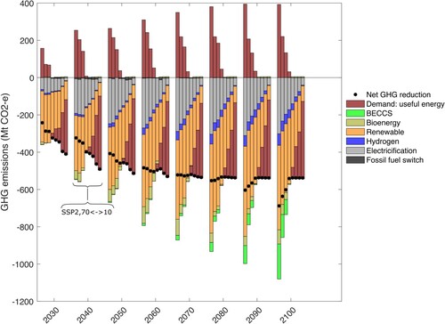
Figure 7. Trajectories of net investment for the eight scenarios in Figures 4–6. We calculate net investment as investment minus stranding of assets. The $10k-utility peak scenario experiences asset stranding worth more than US$ 200bn.

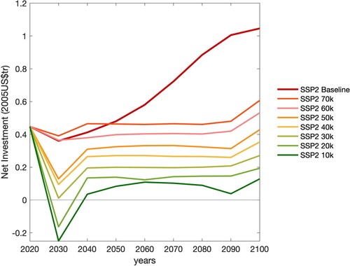
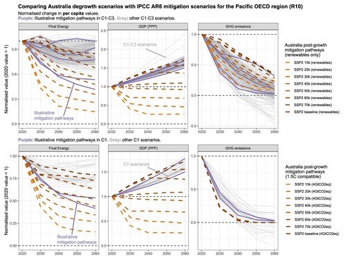
Figure 8. Australian degrowth scenarios compared to the IPCC AR6 mitigation scenarios. Upper row features IPCC climate category C1, C2, and C3 (total: 232 scenarios of 7 model families) in comparison with the renewables only scenarios, and the bottom row features only category C1 (35 scenarios of 6 model families) in comparison with 1.5C compatible scenarios. The AR6 database scenarios are for the IPCC region Pacific OECD (Australia, Japan, and New Zealand - and also South Korea for a minority of scenarios), excluding REMIND scenarios which do not include Australia in this region, and excluding scenarios that did not report population. All values are per capita, normalised in 2020. Values below zero indicate negative values, being negative GHG emissions. GHG emissions here include only CO₂, CH₄, and N₂O for the Australia degrowth scenarios, while it includes a wider set of GHGs in the IPCC scenarios.

Creutzig, F., Roy, J., Lamb, W. F., Azevedo, I. M. L., Bruine de Bruin, W., Dalkmann, H., Edelenbosch, O. Y., Geels, F. W., Grubler, A., Hepburn, C., Hertwich, E. G., Khosla, R., Mattauch, L., Minx, J. C., Ramakrishnan, A., Rao, N. D., Steinberger, J. K., Tavoni, M., Ürge-Vorsatz, D., & Weber, E. U. (2018). Towards demand-side solutions for mitigating climate change. Nature Climate Change, 8(4), 260–263. https://doi.org/10.1038/s41558-018-0121-1

 Web of Science ®Google Scholar

Department of Climate Change, E., the Environment and Water,. (2022). Australia's national greenhouse accounts. Australian Government. Retrieved 12 December from https://ageis.climatechange.gov.au/.

 Google Scholar