149
Views
5
CrossRef citations to date
0
Altmetric
Original Articles

Efficient architectures for sparsely-connected high capacity associative memory models

, &
Pages 163-175 | Received 06 Jan 2007, Published online: 05 Jun 2007

Figures & data

Figure 1. The probability of a connection between any pair of neurons in layer 3 of the rat visual cortex against cell separation. Source: Hellwig, Citation2000, with permission.
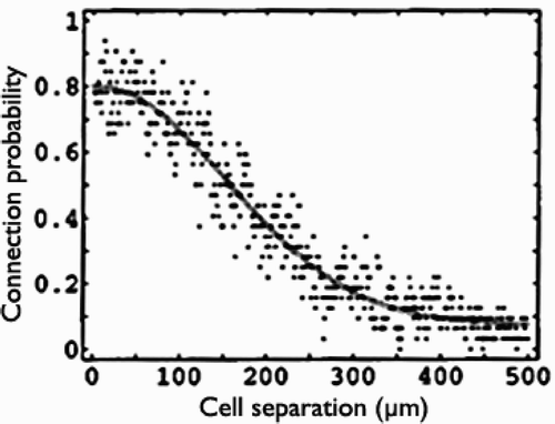
Figure 1. The probability of a connection between any pair of neurons in layer 3 of the rat visual cortex against cell separation. Source: Hellwig, Citation2000, with permission.

Figure 2. (a). Connectivity histogram for a progressively-rewired network at a setting of 50% rewiring, with a class interval of 2. The network consists of 500 units, each with 50 afferent connections per node; (b). Connectivity histogram for a Gaussian network at a σ of 40, and an exponential network at a λ of 0.025, with a class interval of 2. The networks consist of 500 units, each with 50 afferent connections per node; (c). Connectivity histogram for a restricted uniform and restricted linear network, each set to a connection limit of 50% of the maximum connection distance of the network (d lim=125, d max=250). The class interval is 2. The network consists of 500 units, each with 50 afferent connections per node.
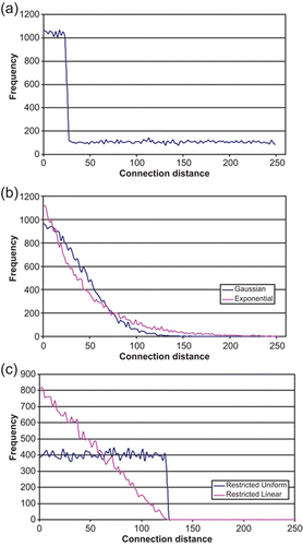
Figure 2. (a). Connectivity histogram for a progressively-rewired network at a setting of 50% rewiring, with a class interval of 2. The network consists of 500 units, each with 50 afferent connections per node; (b). Connectivity histogram for a Gaussian network at a σ of 40, and an exponential network at a λ of 0.025, with a class interval of 2. The networks consist of 500 units, each with 50 afferent connections per node; (c). Connectivity histogram for a restricted uniform and restricted linear network, each set to a connection limit of 50% of the maximum connection distance of the network (d lim=125, d max=250). The class interval is 2. The network consists of 500 units, each with 50 afferent connections per node.

Figure 3. (a) (left). Effective Capacity vs. degree of rewiring. Rewiring beyond about 50% of connections yields little further advantage; (b) (right). Effective Capacity vs. Gaussian σ. Values of σ of 200 and above achieve an Effective Capacity equalling that of the random network. The networks consist of 5000 units, each with 50 afferent connections. Results are averages over 10 runs.
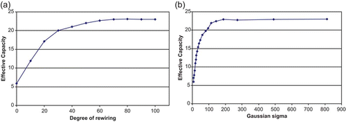
Figure 3. (a) (left). Effective Capacity vs. degree of rewiring. Rewiring beyond about 50% of connections yields little further advantage; (b) (right). Effective Capacity vs. Gaussian σ. Values of σ of 200 and above achieve an Effective Capacity equalling that of the random network. The networks consist of 5000 units, each with 50 afferent connections. Results are averages over 10 runs.

Figure 4. Effective Capacity against mean wiring length for a network of 5000 units with 50 afferent connections per node (connectivity level, k/N, of 0.01). Comparison of Gaussian, exponential and rewiring architectures. Results are averages over 10 runs for each network setting.
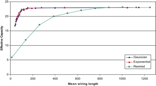
Figure 4. Effective Capacity against mean wiring length for a network of 5000 units with 50 afferent connections per node (connectivity level, k/N, of 0.01). Comparison of Gaussian, exponential and rewiring architectures. Results are averages over 10 runs for each network setting.

Figure 5. Connectivity histogram for a network of 5000 units, each with 50 connections (connectivity level, k/N, of 0.01), comparing Gaussian, exponential and rewiring architectures with the same relatively high Effective Capacity of 22. The class interval is 25.
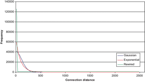
Figure 5. Connectivity histogram for a network of 5000 units, each with 50 connections (connectivity level, k/N, of 0.01), comparing Gaussian, exponential and rewiring architectures with the same relatively high Effective Capacity of 22. The class interval is 25.

Figure 6. Effective Capacity against wiring length for a network of 5000 units, each with 50 afferent connections (connectivity level, k/N, of 0.01). Plots are shown for the Gaussian architecture, the progressively-rewired architecture and the restricted-uniform and restricted-linear architectures. Results are averages over 10 runs for each network setting.
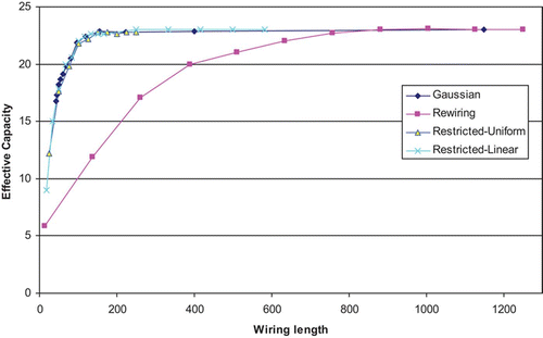
Figure 6. Effective Capacity against wiring length for a network of 5000 units, each with 50 afferent connections (connectivity level, k/N, of 0.01). Plots are shown for the Gaussian architecture, the progressively-rewired architecture and the restricted-uniform and restricted-linear architectures. Results are averages over 10 runs for each network setting.

Figure 7. Effective Capacity against wiring length for a network of 500 units, each with 50 afferent connections (connectivity level, k/N, is 0.1). Plots are shown for the Gaussian architecture, the progressively-rewired architecture and the restricted-uniform and restricted-linear architectures. Results are averages over 50 runs for each network setting.
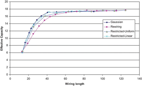
Figure 7. Effective Capacity against wiring length for a network of 500 units, each with 50 afferent connections (connectivity level, k/N, is 0.1). Plots are shown for the Gaussian architecture, the progressively-rewired architecture and the restricted-uniform and restricted-linear architectures. Results are averages over 50 runs for each network setting.

Figure 8. Connectivity histogram for a network of 500 units, each with 50 afferent connections (connectivity level, k/N, is 0.1), comparing the four architectures at the point where Effective Capacity is close to 16 – Gaussian, progressively-rewired, restricted-uniform and restricted-linear. The class interval is 2.
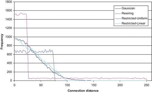
Figure 8. Connectivity histogram for a network of 500 units, each with 50 afferent connections (connectivity level, k/N, is 0.1), comparing the four architectures at the point where Effective Capacity is close to 16 – Gaussian, progressively-rewired, restricted-uniform and restricted-linear. The class interval is 2.

Figure 9. Effective Capacity vs. network size for a network with a fixed number of connections per node, k (=50), for four different connection strategies – a locally-connected network, a random network and ones with Gaussian connectivity distributions with a σ of 30 and with 120 – averages over 10 runs.
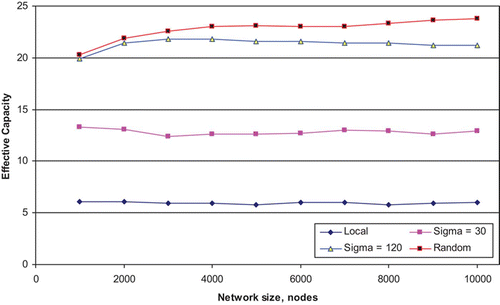
Figure 9. Effective Capacity vs. network size for a network with a fixed number of connections per node, k (=50), for four different connection strategies – a locally-connected network, a random network and ones with Gaussian connectivity distributions with a σ of 30 and with 120 – averages over 10 runs.

Figure 10. (a) Effective Capacity vs. the number of connections per node in a fixed-size network of 5000 units, showing the effect of using different connection strategies – random and local connectivity, a local network with 10% of connections rewired to random nodes and a Gaussian connectivity distribution with a fixed σ of 30. Results are averages over four runs; (b) Effective Capacity vs the number of connections per node in a fixed-size network of 5000 units, showing the effect of using different connection strategies: Random and local connectivity, a local network with 10% of connections rewired to random nodes, and two Gaussian connectivity distributions whose value of σ is made proportional to k, the number of connections per node (in one case σ is set to 2.4 k and in the other to 0.6 k). Results are averages over four runs.
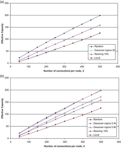
Figure 10. (a) Effective Capacity vs. the number of connections per node in a fixed-size network of 5000 units, showing the effect of using different connection strategies – random and local connectivity, a local network with 10% of connections rewired to random nodes and a Gaussian connectivity distribution with a fixed σ of 30. Results are averages over four runs; (b) Effective Capacity vs the number of connections per node in a fixed-size network of 5000 units, showing the effect of using different connection strategies: Random and local connectivity, a local network with 10% of connections rewired to random nodes, and two Gaussian connectivity distributions whose value of σ is made proportional to k, the number of connections per node (in one case σ is set to 2.4 k and in the other to 0.6 k). Results are averages over four runs.

Figure 11. Effective Capacity of networks based on different connection strategies, as network size is increased from 1000, while keeping a fixed connectivity level, k/N, of 0.1. The results are averages over four runs.
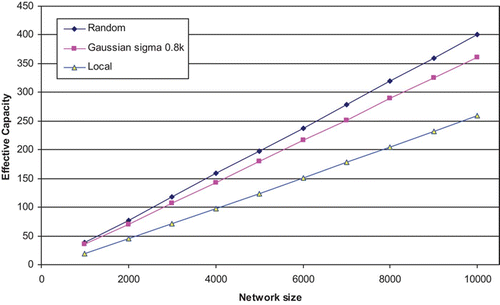
Figure 11. Effective Capacity of networks based on different connection strategies, as network size is increased from 1000, while keeping a fixed connectivity level, k/N, of 0.1. The results are averages over four runs.

Figure 12. Effective Capacity of networks based on different connection strategies, as network size is increased from 1000, while keeping a fixed connectivity level, k/N, of 0.01. The results are averages over four runs.
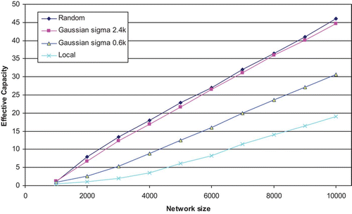
Figure 12. Effective Capacity of networks based on different connection strategies, as network size is increased from 1000, while keeping a fixed connectivity level, k/N, of 0.01. The results are averages over four runs.

Figure 13. Convergence time (measured in cycles) vs. the degree of noise applied to each pattern in a network of 500 nodes, each with 50 afferent connections. A range of architectures is represented, each of whose parameters gives rise to an Effective Capacity of 16. Each network is trained on 16 patterns, thus the point at which the noise is 60% corresponds to the exact conditions of earlier Effective Capacity measurements. Results are averages over 50 runs.
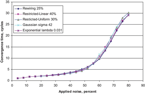
Figure 13. Convergence time (measured in cycles) vs. the degree of noise applied to each pattern in a network of 500 nodes, each with 50 afferent connections. A range of architectures is represented, each of whose parameters gives rise to an Effective Capacity of 16. Each network is trained on 16 patterns, thus the point at which the noise is 60% corresponds to the exact conditions of earlier Effective Capacity measurements. Results are averages over 50 runs.

Figure 14. Convergence time (measured in cycles) vs. the degree of noise applied to each pattern in a network of 5000 nodes, each with 50 afferent connections. A range of architectures is represented, each of whose parameters gives rise to an Effective Capacity of 20. Each network is trained on 20 patterns, thus the point at which the noise is 60% corresponds to the exact conditions of earlier Effective Capacity measurements. Results are averages over 10 runs.
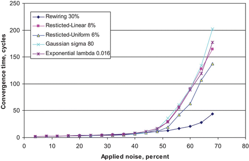
Figure 14. Convergence time (measured in cycles) vs. the degree of noise applied to each pattern in a network of 5000 nodes, each with 50 afferent connections. A range of architectures is represented, each of whose parameters gives rise to an Effective Capacity of 20. Each network is trained on 20 patterns, thus the point at which the noise is 60% corresponds to the exact conditions of earlier Effective Capacity measurements. Results are averages over 10 runs.

Reprints and Corporate Permissions

Please note: Selecting permissions does not provide access to the full text of the article, please see our help page How do I view content?

To request a reprint or corporate permissions for this article, please click on the relevant link below:

Academic Permissions

Please note: Selecting permissions does not provide access to the full text of the article, please see our help page How do I view content?

Obtain permissions instantly via Rightslink by clicking on the button below:

If you are unable to obtain permissions via Rightslink, please complete and submit this Permissions form. For more information, please visit our Permissions help page.