The dual-route hypothesis: evaluating a neurocomputational model of fear conditioning in rats

Figures & data

Figure 1. Dual-route pathway for sub-cortical and cortical stimulus processing convergence on the amygdala.

Figure 2. Armony et al. (1995, 1997a b) original model architecture. The anatomical modules identified as being pertinent to the fear circuitry in the rat brain are represented here along with the number of units contained and their feed-forward, excitatory connections to other modules. Connections between modules are modified through an extended Hebbian learning rule. CS, conditioned stimulus; MGv, ventral division of the medial geniculate body (MGB); MGm, medial division of the MGB; PIN, posterior intralaminar nucleus. This model depicts a particular unit number configuration of the form [a b c d] where a, MGv, b, PIN/MGm, c, auditory cortex and d, amygdala. This particular cell unit configuration is thus: 8 3 8 3 as used by Armony et al. (1995).

Figure 3. Single amygdala unit receptive field (RF) in the Armony model. (A) A single unit from Armony et al. (1995). (B) Single unit from our replication of that model. Top: both show that the amygdala unit establishes a broad RF with a peak best frequency (BF) during the development phase, which shifts to the conditioned stimulus (CS) after the conditioning phase. Bottom: the difference between the RFs at the end of each phase shows clearly the shift in peak activation to the CS following the conditioning phase. Armony, J.L., Servan-Schreiber, D., Cohen J.D., and LeDoux, J.E. (1995), ‘An anatomically Constrained Neural Network Model of Fear Conditioning,’ Behavioral Neuroscience, 109, 246–257. Reprinted with permission.)

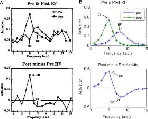
Figure 4. (A) The behavioural response (summed total amygdala activation) pre- and post-conditioning from Armony et al. (1995). (B) The behavioural response pre- and post-conditioning from our replication of the model; the points are the mean of 10 simulation runs, shown±S.E., emphasising the robustness of the results. Our simulations replicate the broad response pre-conditioning, and the peaked response, centred on the conditioned stimulus (CS) input, post-conditioning. Note that our activation values are normalised by the number of amygdala units to allow plotting on the same scale as the Armony et al. results. Results of an auditory cortex lesioned model are also depicted for completeness. (Armony, J.L., Servan-Schreiber, D., Cohen, J.D., and LeDoux, J.E. (1995) ‘An Anatomically Constrained Neural Network Model of Fear Conditioning,’ Behavioral Neuroscience, 109, 246–257. Reprinted with permission.)

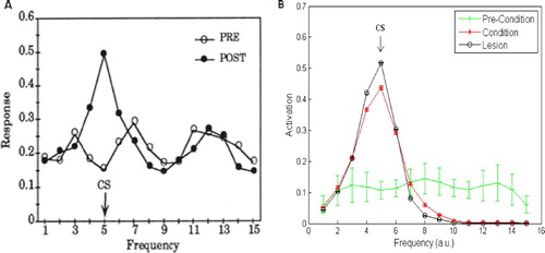
Figure 5. Replication of the Armony et al. (1997b) model. (A) From Armony et al. (1997b), shows the behavioural response (total amygdala activation) to the CS tone pre- and post-conditioning in both control and lesion conditions. (B) The stimulus generalisation gradient (SGG) – the percentage change at each input from the development phase to the conditioning phase. Mean and error bars were from five repetitions of the simulations. (C,D) Corresponding results from our own simulations, showing that we replicated their main findings; we show here the behavioural response for more than just the CS in (C) to demonstrate that the 1997 Armony model could also generalise its response. Mean and error bars are from 10 repetitions of the simulations. (Armony, J.L., Servan-Schreiber, D., Romanski, L.M., Cohen, J.D., and LeDoux, J.E. (1997) ‘Stimulus Generalization of Fear Responses: Effects of Auditory Cortex Lesions in a Computational Model and in Rats,’ Cerebral Cortex, 7, 157–165. Reprinted with permission from Oxford Journals, Oxford University Press.)

Figure 6. Responses of the Armony model to changes in the number of units per module. The left column shows the behavioural responses (summed and normalised total activation of all amygdala units) pre- and post-conditioning for the control and lesion conditions. The right column shows the stimulus generalisation gradient (SGG) for the same conditions. (A,B): Configuration 1, 24 3 24 3; (C,D): configuration 2, 3 24 3 24. In both configurations the model produced stable receptive fields and a corresponding pre-conditioning behavioural response, a shift in peak behavioural response to the CS tone, and a SGG that showed the model generalised its learned response to tones close to the CS in input space (the CS was always pattern 5). Mean values and error bars were taken from 10 repetitions of the simulations with different initial random weights.

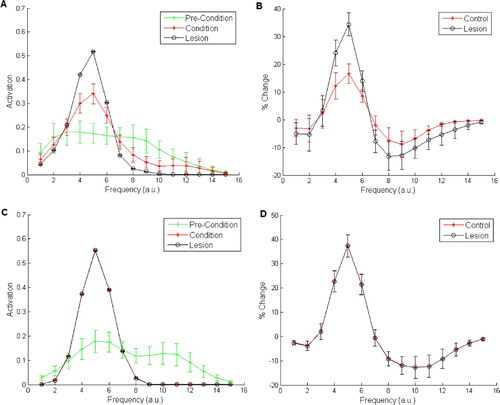
Figure 7. Unit activity (left column) and behavioural responses (right column) in the Armony model, when using a difficult-to-condition-CS. (A,B) Cellular activity and behavioural responses where population coding is used in a single simulation run. (A) shows four example units out of the 10 used – 2–4 are representative of units 5–10. (C) shows the same respective phenomena in the same testing conditions for a non-population coding network – note, the single unit in this case also represents the behavioural response of the network.

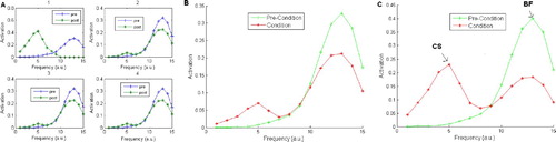
Figure 8. Stimulus generalisation gradients for: (A) a single unit network; (B) a single module network; and (C) for an intact thalamo-amygdala network. In the network tested in (C) the sub-cortical modules contained 10 units. Testing in the conditioning phase was always recorded after five epochs. The development phase was for 300 epochs. Means and standard errors were taken from 20 simulations.

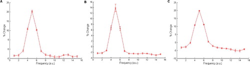
Figure 9. Total network output for MGv-lesioned and auditory cortex-lesioned models respectively, where Armony et al. (1995) parameters are adhered to including configuration 8 3 8 3. (A) Output for the MGv-lesioned network. (B) Output for the auditory cortex-lesioned network. The two conditions show means and error bars from 20 simulations, 300 epochs in the development phase, five epochs in the conditioning and lesioning phase. The grey horizontal line is used to emphasise the small difference in behavioural response between the two conditions.

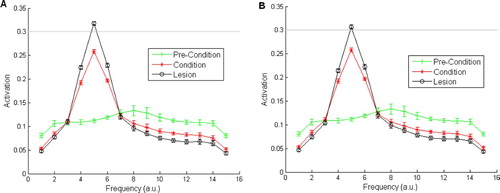
Figure 10. Stimulus generalisation gradients for the pre-development MGv-lesioned model – parameters of Armony et al. (1995) are adhered to including configuration 8 3 8 3, auditory cortex is lesioned in the post-conditioning. (A) The SGG after five epochs in the conditioning and lesioning phase. (B) The SGG after 300 epochs in the conditioning and lesioning phase. Means and standard errors were taken over 20 simulations, 300 epochs were used in the development phase.

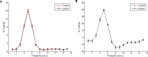
Figure 11. Stimulus generalisation gradients for pure feed-forward and dual-route (MGv-lesioned) processing models using configuration 10 10 10 10 – otherwise Armony et al. (1995) parameters. (A) The SGG for the pure feed-forward processing model. (B) The SGG for the dual-route (MGv-lesioned) processing model. Means and standard errors taken over 20 simulations with 300 epochs for development phase and five epochs in the conditioning phase. The grey horizontal line is used to emphasise the small difference in behavioural response between the two conditions.

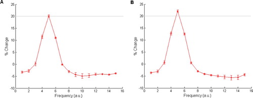
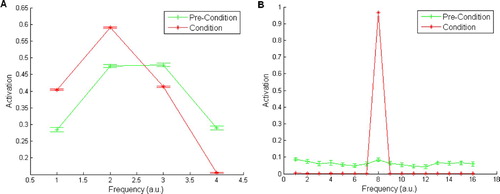
Figure 12. The effect of changing unit connectivity type in the Armony model. (A) Full connectivity model behavioural responses (summed total amygdala activation), with parameters from Armony et al. (1995) with four units per module. (B) Behavioural responses from a unit-to-unit connectivity version of the model with the same total number of connections, that is, 16 units per module, respectively. In this case the model had a small behavioural response after the development phase, indicating the presence of receptive fields, but the learned response to the CS input after the conditioning phase removed all but the CS field. Total activation is normalised by the number of connections from the input stimulus to its connecting layers. Mean values and error bars were taken from 10 repetitions of the simulations with different initial random weights.

Armony , J. L. , Servan-Schreiber , D. , Cohen , J. D. and LeDoux , J. E. 1995 . An Anatomically Constrained Neural Network Model of Fear Conditioning . Behavioral Neuroscience , 109 : 246 – 257 .

 PubMed Web of Science ®Google Scholar

Armony , J. L. , Servan-Schreiber , D. , Cohen , J. D. and LeDoux , J. E. 1997a . Computational Modeling of Emotion: Explorations Through the Anatomy and Physiology of Fear Conditioning . Trends in Cognitive Science , 1 : 28 – 34 .

 PubMed Web of Science ®Google Scholar

Armony , J. L. , Servan-Schreiber , D. , Romanski , L. M. , Cohen , J. D. and LeDoux , J. E. 1997b . Stimulus Generalization of Fear Responses: Effects of Auditory Cortex Lesions in a Computational Model and in Rats . Cerebral Cortex , 7 : 157 – 165 .

 PubMed Web of Science ®Google Scholar

LeDoux , J. E. 1990 . “ Information Flow from Sensation to Emotion: Plasticity in the Neural Computation of Stimulus Value ” . In Learning and Computational Neuroscience: Foundations of Adaptive Networks , Edited by: Gabriel , M. and Moore , J. 3 – 51 . Cambridge , MA : MIT Press .

 Google Scholar

Bordi , F. and LeDoux , J. E. 1994 . Response Properties of Single Units in Areas of Rat Auditory Thalamus that Project to the Amygdala . Experimental Brain Research , 98 : 275 – 286 .

 PubMed Web of Science ®Google Scholar