Figures & data
Figure 1. (Top) Recognition depicted as the formation of a brain state (drawn as lightning on the forehead) that becomes correlated with a physical event (lightning). (Middle) Learning the association between one event (lightning) and its successor (thunder) by linking the brain states that correlate with each. (Bottom) Declarative prediction entails recognising one event (lightning) and forming the succeeding brain state for thunder prior to (or even in the absence of) the real-world event with which it correlates.
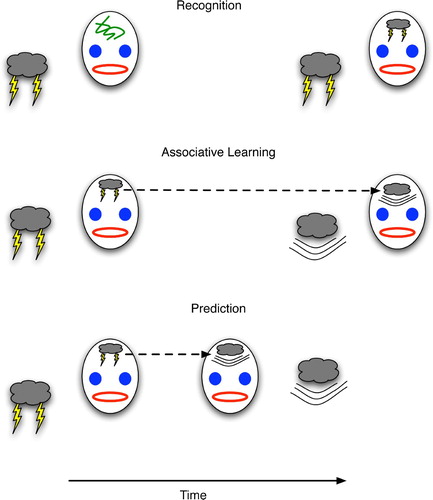
Figure 2. Procedural prediction, wherein the agent's actions indicate specific knowledge of a future world state, even though the agent (monkey) has no explicit brain state that strongly correlates with the world state. The agent's ear-covering behaviour can easily lead an observer to infer that the agent has the strongly correlated brain state, i.e. explicit knowledge of the upcoming thunder.
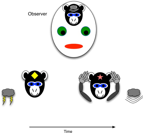
Figure 3. The basic organisation of the cerebellum, an abstraction and combination of more complex diagrams in Bear et al. Citation(2001), originally appearing in Downing Citation(2007).
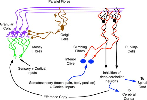
Figure 4. Granular cells realise sparse coding for temporally blended contexts. Events (e) of various temporal origin (denoted by subscripts) simultaneously activate granular cells due to differential delays – roughly depicted by line length, with longer lines denoting events that occurred further in the past – along mossy fibres.
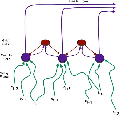
Figure 5. Temporally mixed sensory and proprioceptive experiences of a baseball outfielder. These form a context for increasing vertical foot plant while accelerating to catch a fly ball.
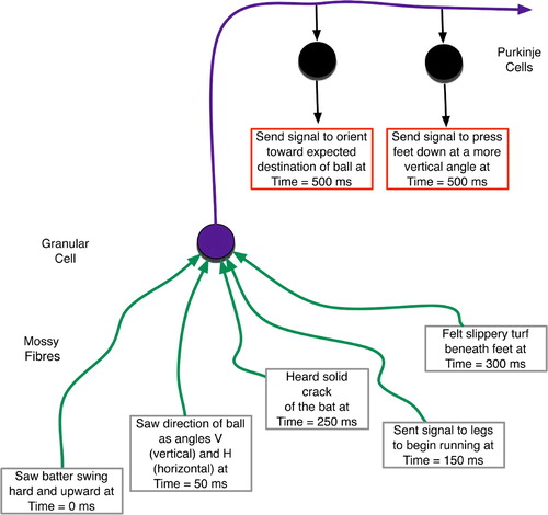
Figure 6. The temporal scope of cerebellar decision-making. Context from the past affects present action choices whose actions are realised in the future and whose consequences are perceived even further in the future.
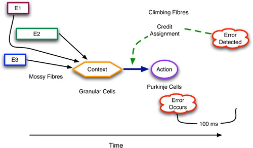
Figure 7. Cerebellar eligibility traces, drawn as rectangles on the condition–action arcs, with taller rectangles denoting higher eligibility. Synapses are most eligible for modification approximately 100 s after they transmit an action potential.
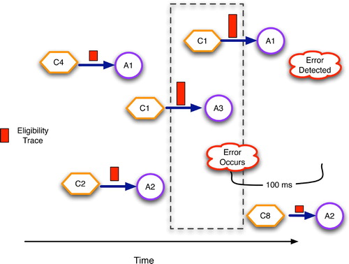
Figure 8. Regressive prediction: the agent recognises earlier and earlier indicators of the emotive event.
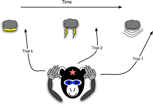
Figure 9. Basic anatomy of the basal ganglia in one hemisphere, shown as a coronal cross-section. Based on diagrams in Bear et al. Citation(2001) and Prescott, Gurney and Redgrave Citation(2003).
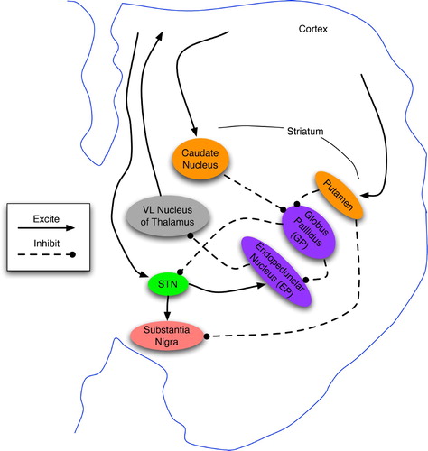
Figure 10. Functional topology of the basal ganglia and their main inputs, derived from the text and diagrams in Houk Citation(1995), Houk et al. Citation(1995a), Prescott et al. Citation(2003) and Graybiel and Saka Citation(2004). The actor denotes the direct outputs of the BG: EP and SNr, whereas the critic consists of the diffuse neuromodulatory output from SNc. Matriosomes are primarily gateways to the actor circuit, whereas striosomes have direct-pathway links to both actors and critics.
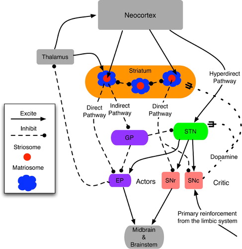
Figure 11. Temporal regression of predictive competence using eligibility traces and reinforcement signals in the basal ganglia. C2 and C3 are contexts detected by the striatum and STN, whereas A2 and A3 are accepted/chosen versions of C2 and C3, respectively.
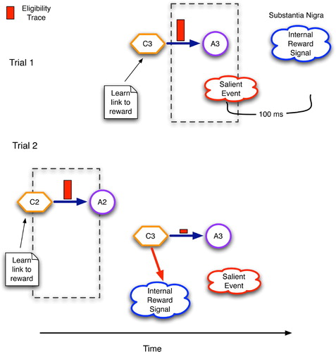
Figure 12. The implicit reinforcement learning of sequence X→Y→Z→R. Horizontal plots are the time series activation levels for the substantia nigra pars compacta (SNc). Solid arrows denote excitatory effects upon the SNc, whereas round heads represent the delayed inhibition. Dashed arrows portray the learning of a new context governed by the SNc's dopamine signal.
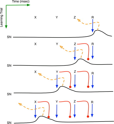
Figure 13. The Generic Declarative Prediction Network (GDPN). Neurons A, B and C serve as low-level detectors for stimuli A, B and C, and W–Z represent neurons at a higher level. Only the axonal projections from X are shown, although W, Y and Z have similar links to the lower level. The T1–T4 diamonds represent time steps, and S1 and S2 denote important synapses, as discussed further in the text.
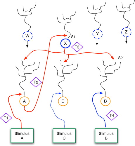
Figure 14. (Top) Top-down, predictive, distal and bottom-up, sensory, proximal inputs to a neuron. (Bottom) Changes in synaptic strength as a function of post-synaptic stimulation intensity.
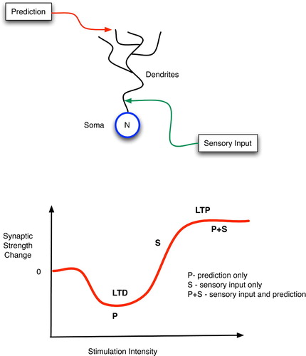
Figure 15. Abstract view of cortical columns and top-down versus bottom-up information flow. Bottom-up flow (solid lines) goes from layers 2 and 3 of the sending column to layer 4 of the higher-level column, but with additional synapses on to the large pyramidals in layers 5 and 6 (pentagons). In the top-down pathway (dotted line), large pyramidals output to layer 1 of lower-level columns, with the signal eventually reaching layers 5 and 6 via either the layer 2–3 relays or directly via long dendrites from the large pyramidals.
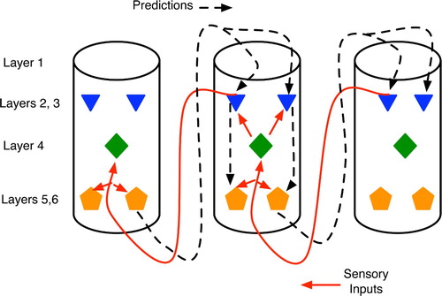
Figure 16. (Top) Basic anatomy of the mammalian hippocampus. (Bottom) Primary hippocampal areas and their connectivity. Box dimensions roughly illustrate relative sizes of neural populations in each area; all connections are excitatory. Based on pictures and diagrams in Burgess and O'Keefe Citation(1994), Rolls and Treves Citation(1998) and Andersen et al. Citation(2007).
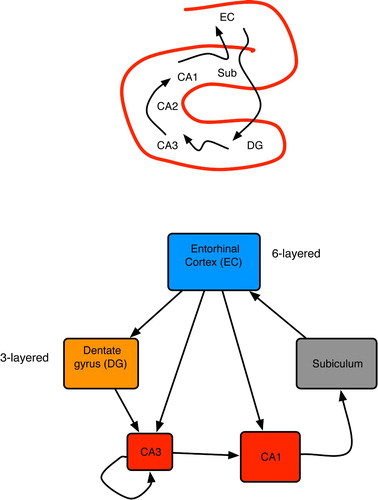
Figure 17. Two main sources of input to CA3 neurons: proximal connections from the dentate gyrus and distal, recurrent inputs from CA3 itself. Each CA3 neuron has recurrent links to 1–5% of the others (Rolls and Treves Citation1998; Andersen et al. Citation2007).
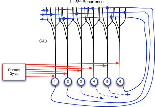
Figure 18. Learning a predictive association in the hippocampus. In these diagrams: large arrows extending from DG indicate active output ports; and CA3 neurons are separated into three groups for explanatory purposes only. (Top left) Input of pattern 1–3 from the dentate gyrus via proximal synapses on to CA3 pyramidals. (Top right) Context neurons send distal monitoring signals to their recurrent connections and to themselves. This causes weak activation of distal dendrites throughout CA3 and incites autocatalytic learning within the 4–5 context. (Bottom left) Distal monitoring inputs from the 4–5 context coincide with DG-forced firing of neurons 2 and 6 (as a consequence of event E2). This leads to LTP at the distal synapses of neurons 2 and 6. (Bottom right) Using the learned association between events E1 and E2: when E1 occurs, 4–5 context neurons and then neurons 2 and 6 fire, thus predicting the future occurrence of E2.
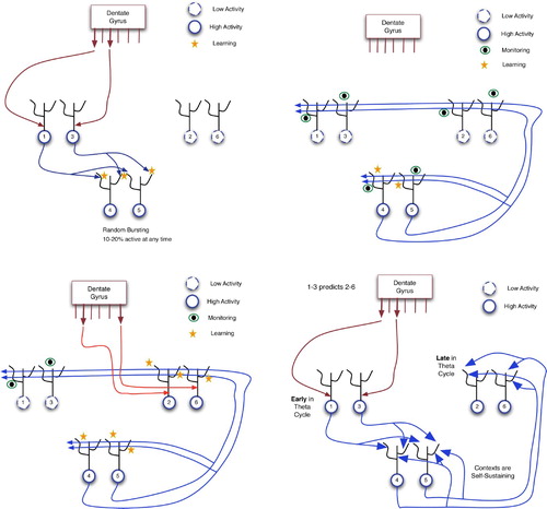
Figure 19. Regions and connections of the thalamocortical loop germane to a discussion of predictive models, based on descriptions in Rodriguez, Whitson and Granger Citation(2004). The cortex is divided into regions, vertical columns, and the six well-known horizontal layers. Each core cell maps to layer 4 of a specific cortical column and receives feedback from layer 6. Matrix cells receive cortical afferents from layer 5 and send signals to the layer 1 dendritic mats of many columns.
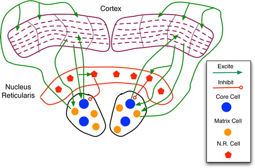
Figure 20. Sketch of thalamocortical loops for three columns of a cortical region. Core, matrix and nucleus reticularis (NR) cells are separated into three modules for illustrative purposes. The main types (but not all instances) of connections are drawn. Within a column, the key connections are: entry layer 4 links to layers 2 and 3; layer 2–3 stimulation of layers 5 and 6; and layer 1 excitation of layers 2, 3 and 5. In general, the column is considered active when layer 5 and 6 neurons fire at high frequency.
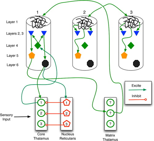
Figure 21. Learning of a predictive sequence in the thalamocortical circuit. Only the main active connections are shown. (a) Entry of stimulus 1 stimulates the corresponding core thalamus neuron and cortical column, as well as a random matrix thalamus neuron. (b) Matrix stimulation leads to distal monitoring of diverse cortical columns. (c) Entry of stimulus 2 adds proximal stimulation to (already distally stimulated) cortical column 2, producing distal synaptic strengthening. (d) In future trials, stimulus 1 leads to excitation of column 1, then 2, thus embodying a prediction of stimulus 2.
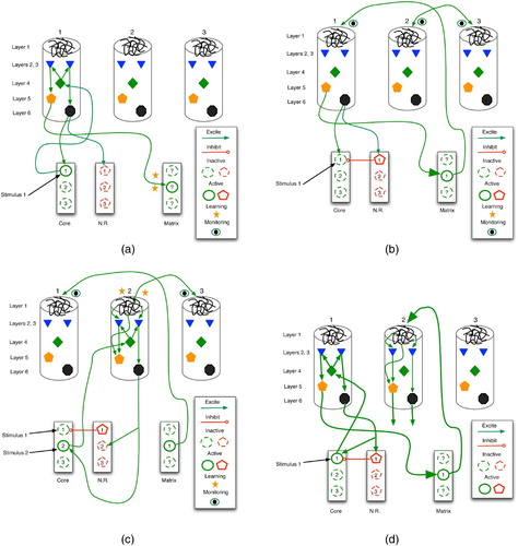
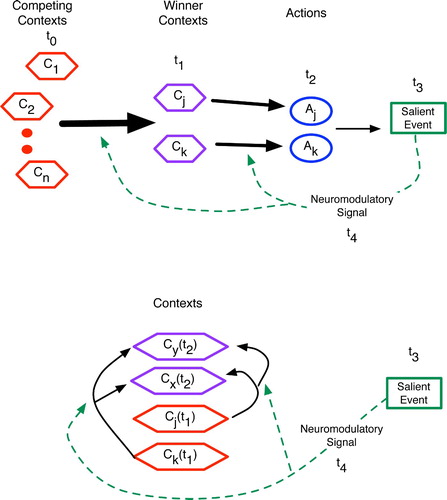
Figure 22. Abstract comparison of the procedural (top) and declarative (bottom) predictive mechanisms, with relative time points given as t 0 - t 4 and vertical cell columns indicating brain regions. (Top) In procedural prediction, neural patterns corresponding to competing contexts, winning contexts and proposed actions have distinct spatial locations in the brain. Salient events and the ensuing feedback (via neuromodulators) then alter synapses between these regions, such as between granular cell contexts of the cerebellum and the action-regulating Purkinje cells. Similar spatial localisation occurs in the basal ganglia. (Bottom) In declarative areas such as the hippocampus, cortex and thalamocortical system, active patterns have considerably more spatial overlap such that neuromodulatory feedback affects recurrent (often distal) connections within a region. The competition among contexts thus occurs in place.