Figures & data
Figure 1. The experimental set-up. Two participants face each other in a 600-unit-long 1-D environment that wraps around at the edges. Note that a participant's receptor field (white bar) can encounter three different objects (grey bars): a static object (located at 148 or 448, depending on the participant), the other participant's avatar (coinciding with the location of its receptor field) and the other's ‘shadow’ (attached to the other's avatar via a rigid link of 48 units). As all objects have the same width (4 units) they cannot be told apart by any inherent differences between their appearances (they all give rise to the same all-or-nothing tactile response whenever a participant's avatar makes contact with them).

Figure 2. The CTRNN controller used for experimental set-up 1. Circles represent CTRNN nodes with time constants τ i , square-tailed arrows represent bias connections b i , diamond-tailed arrows represent weighted input connections Iw i , normal arrows represent motor outputs z i (L-M, left motor; R-M, right motor) and circle-headed lines represent weighted inter-node connections w ij (including self-connections). Negative connections are depicted as dashed lines, whereas positive connections are solid. The size of the arrows is roughly proportional to the weight strength of the connection, while the line width of the circles is roughly proportional to the decay speed of the node.
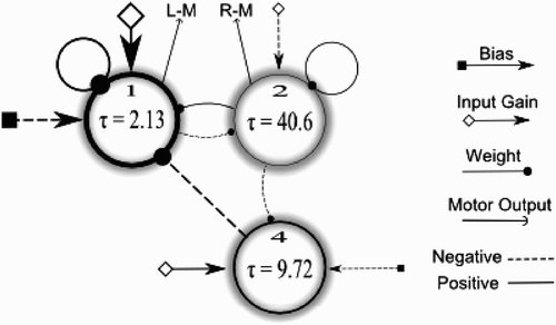
Figure 3. Graphical representation of fitness scores achieved at each possible combination of starting positions for agent ‘up’ (x-axis) and agent ‘down’ (y-axis). Note that the axes wrap around owing to the 1-D circular shape of the virtual environment. Fitness scores range from 0.60 to 0.96 with an average of 0.87. See text for an explanation of the different regions.
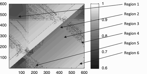
Figure 4. Illustration of the behaviour of the agents during a representative trial starting from point (100, 500) with a score of 0.74. They first encounter their respective static objects, then continue searching, and finally locate each other and establish perceptual crossing until the end of the run (16,000 time steps). (a) The position of the agents and objects in the 1-D environment over time. (b) The sigmoid node outputs of agent ‘up’ over time. (c) The sensorimotor behaviour agent ‘up’ over time. Note that a change of receptor field status reaches the agent's controller only after a delay of 25 units of time (250 steps).
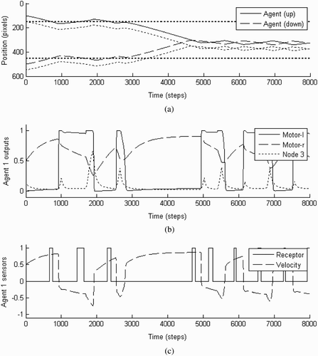
Figure 5. Graphical representation of fitness scores achieved at each possible combination of starting positions for agent ‘up’ (x-axis) and agent ‘down’ (y-axis). Note that the axes wrap around owing to the 1-D circular shape of the virtual environment. Fitness scores range from 0.40 to 0.965 with an average score of 0.87.
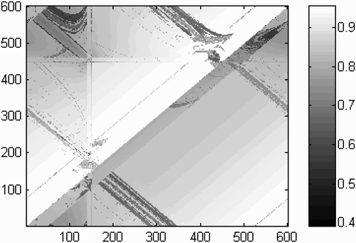
Figure 6. Illustration of the behaviour of the agents during a representative trial starting from point (100, 500). The experimental set-up is the same as in , except that the input to the receptor fields of the agents has been exchanged between them. Fitness score: 0.71.
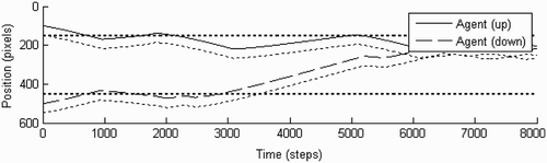
Figure 7. Graphical representation of fitness scores achieved at each possible combination of starting positions for agent ‘up’ (x-axis) and agent ‘down’ (y-axis). Note that the axes wrap around owing to the 1-D circular shape of the virtual environment. (a) Normal condition. Fitness scores range from 0.09 to 0.94 with an average of 0.80. (b) Swapped receptor fields. Fitness scores range from 0.06 to 0.94 with an average of 0.80.
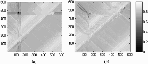
Figure 8. Illustration of the behaviour of the agents during a representative trial starting from point (100, 500) with a score of 0.72. They first encounter their respective static objects, then continue searching, and finally locate each other and establish perceptual crossing until the end of the run (16,000 time steps). (a) The position of the agents and objects in the 1-D environment over time. (b) The node outputs of agent ‘up’ over time. (c) The status of the receptor field and the velocity of agent ‘up’ over time. Note that a change of receptor field status reaches the agent's controller only after a delay of 25 units of time (250 steps).
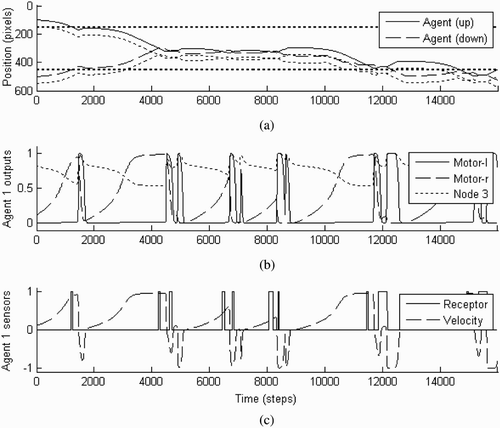
Figure 9. Diagram of a hypothetical circuit that could explain the discriminatory behaviour of the agents. D1 and D2 are delays (total delay: 25 units of time), ∫ I dt is the integral of the input signal I for K units of time, T1 and T2 are thresholds, and G1 and G2 are output gains.
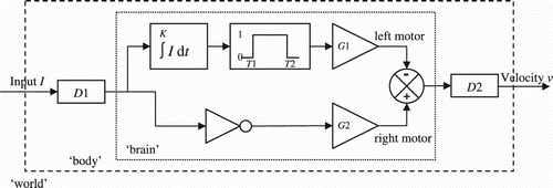
Figure 10. The attractor landscape for the CTRNN shown in . The node activations were initialised 50 times to random activation values drawn from the trial shown in , and the network was allowed to settle for 8000 time steps. The axes (motor-l, motor-r, node 3) represent the sigmoid output of the three CTRNN nodes. The input was either (a) set to zero, which revealed a fixed point attractor at (0.04, 0.91, 0.02), or (b) set to unity, which revealed a fixed point attractor at (0.98, 0.02, 0.88). The attractors are represented by an asterisk. Input-driven switching between the two attractors results in a hysteresis of motor outputs.
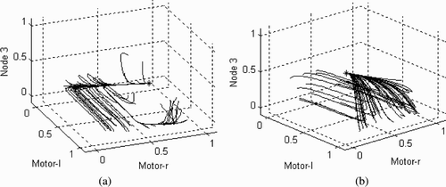
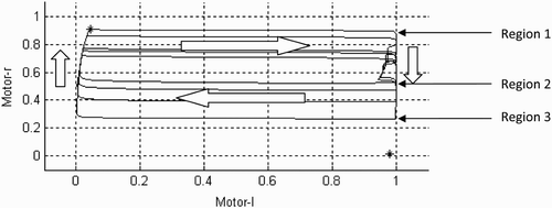
Figure 11. Change of state between the left and right motors during the trial that was shown in . Arrows indicate direction and relative velocity of trajectories (i.e. long arrows, fast trajectories; short arrows, slow trajectories). For an explanation of regions 1–2 and 2–3 on the left-hand side of the state space, see the text.