247
Views
2
CrossRef citations to date
0
Altmetric
Original Articles

Macroscopic definition of distributed swarm morphogenesis

, &
Pages 162-192 | Received 29 Oct 2012, Accepted 11 Apr 2013, Published online: 13 May 2013

Figures & data

Figure 1. Basic structure of the simulated robots. Each robot can be assembled on each of its sides. The robot can move in any direction on the x–y axis.
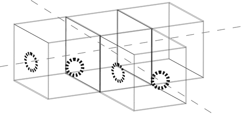
Figure 1. Basic structure of the simulated robots. Each robot can be assembled on each of its sides. The robot can move in any direction on the x–y axis.

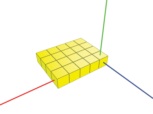
Figure 2. Morphology generated with the language defined in .

Figure 2. Morphology generated with the language defined in Figure 3.

Figure 3. Swarm line arrangement language. i determines the number of robots that are part of the assembly and hence the line length. In addition, the sequence of words generated up to i=3 is presented. Parentheses in this sequence show where the last symbol was replaced by the interpreter.
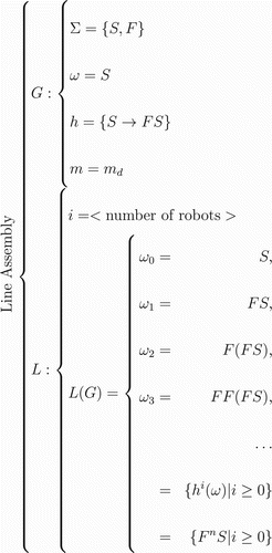
Figure 3. Swarm line arrangement language. i determines the number of robots that are part of the assembly and hence the line length. In addition, the sequence of words generated up to i=3 is presented. Parentheses in this sequence show where the last symbol was replaced by the interpreter.

Figure 4. An example of morphology generated with the language defined in .

Figure 4. An example of morphology generated with the language defined in Figure 5.

Figure 5. Language for the generation of rectangular assemblies. i determines the height of the assembly. This language definition uses the repetition operator to define the width of the rectangle. The size of the assembly is limited, because i∈ℤ, forces the width to be even. Parentheses in this sequence show where the last symbol was replaced by the interpreter.
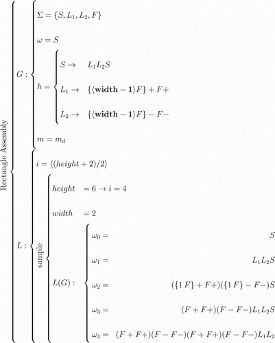
Figure 5. Language for the generation of rectangular assemblies. i determines the height of the assembly. This language definition uses the repetition operator to define the width of the rectangle. The size of the assembly is limited, because i∈ℤ, forces the width to be even. Parentheses in this sequence show where the last symbol was replaced by the interpreter.

Figure 6. Sequential order of assembly for a 5×4 rectangle. The thickness of the lines indicates assemblies within the same rule.
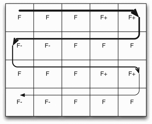
Figure 6. Sequential order of assembly for a 5×4 rectangle. The thickness of the lines indicates assemblies within the same rule.

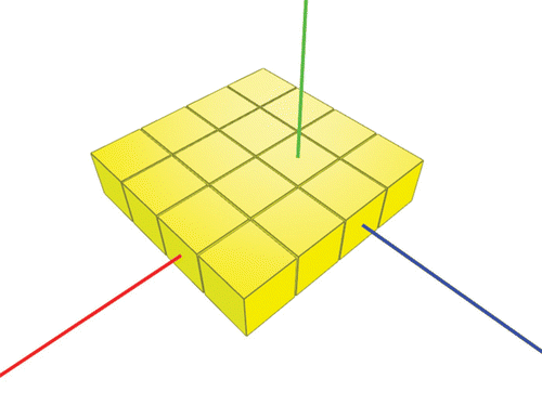
Figure 7. Morphology generated with the language defined in .

Figure 7. Morphology generated with the language defined in Figure 8.

Figure 8. Language for generating square assemblies. We present a set of sample words obtained from this language for i=3.
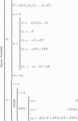
Figure 8. Language for generating square assemblies. We present a set of sample words obtained from this language for i=3.

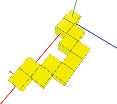
Figure 9. Example of morphology generated with the language defined in .

Figure 9. Example of morphology generated with the language defined in Figure 10.

Figure 10. Language for generating arrow-shaped assemblies. Parentheses in this sequence show where the last symbol was replaced by the interpreter. Recursion factor i determines the rows that will define the arrow.
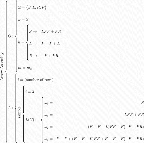
Figure 10. Language for generating arrow-shaped assemblies. Parentheses in this sequence show where the last symbol was replaced by the interpreter. Recursion factor i determines the rows that will define the arrow.

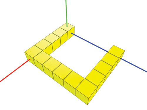
Figure 11. Example of morphology generated with the language defined in .

Figure 11. Example of morphology generated with the language defined in Figure 12.

Figure 12. Language for the generation of horseshoe-shaped assemblies. Parentheses in this sequence show where the last symbol was replaced by the interpreter. Recursion factor i determines the length of a horseshoe segment.
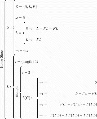
Figure 12. Language for the generation of horseshoe-shaped assemblies. Parentheses in this sequence show where the last symbol was replaced by the interpreter. Recursion factor i determines the length of a horseshoe segment.

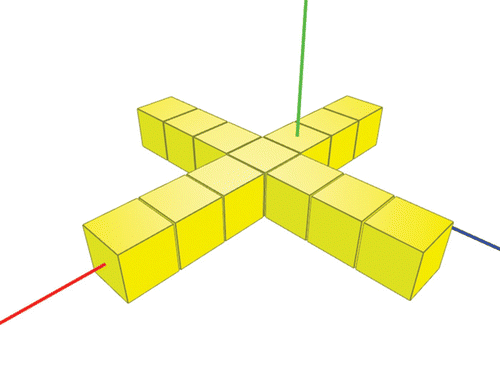
Figure 13. Sample morphology generated by the language defined in .

Figure 13. Sample morphology generated by the language defined in Figure 14.

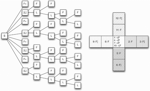
Figure 14. Language for the generation of star-shaped assemblies. In this case, we use a turtle interpreter with a stack to be able to generate Hamiltonian paths. Parentheses in this sequence show where the last symbol was replaced by the interpreter.
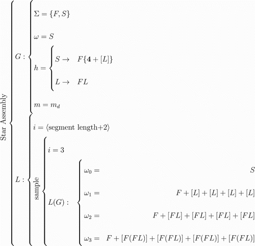
Figure 14. Language for the generation of star-shaped assemblies. In this case, we use a turtle interpreter with a stack to be able to generate Hamiltonian paths. Parentheses in this sequence show where the last symbol was replaced by the interpreter.

Figure 15. Distributed assembly with a rectangular shape using the LSDA algorithm with the language presented in for a width of five robots and a height of four. In the upper figure, the communication structure of the robot that starts the assembly process is shown. Below, we specify the steps of the assembly process for each of the zones (A, B, C, D, E and F) as defined in the upper diagram. The white-tipped arrows of the robots define the passive connection vector, black-tipped arrows the active.
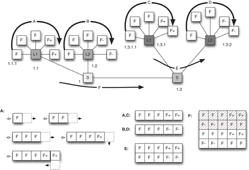
Figure 15. Distributed assembly with a rectangular shape using the LSDA algorithm with the language presented in Figure 5 for a width of five robots and a height of four. In the upper figure, the communication structure of the robot that starts the assembly process is shown. Below, we specify the steps of the assembly process for each of the zones (A, B, C, D, E and F) as defined in the upper diagram. The white-tipped arrows of the robots define the passive connection vector, black-tipped arrows the active.

Figure 16. Distributed assembly of a square-shaped form using the LSDA algorithm with the language presented in for a cube of four robots.
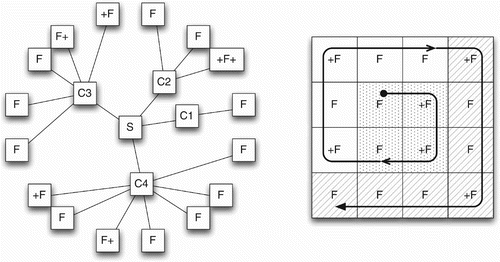
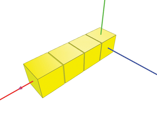
Figure 16. Distributed assembly of a square-shaped form using the LSDA algorithm with the language presented in Figure 8 for a cube of four robots.

Figure 17. Distributed assembly of a star-shaped form using LSDA algorithm with the language presented in for i=5.

Figure 17. Distributed assembly of a star-shaped form using LSDA algorithm with the language presented in Figure 14 for i=5.

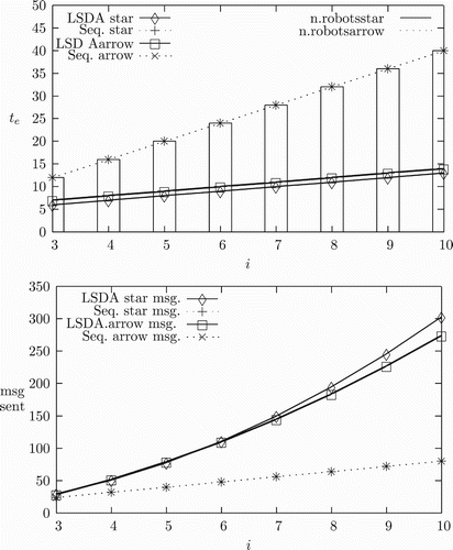
Figure 18. Comparison of assembly time (top) and sent messages (below) for LSDA and sequential swarm system for star and arrow assembly. The number of robots that define the final structure for each iteration level i is also shown.

Figure 18. Comparison of assembly time (top) and sent messages (below) for LSDA and sequential swarm system for star and arrow assembly. The number of robots that define the final structure for each iteration level i is also shown.

Reprints and Corporate Permissions

Please note: Selecting permissions does not provide access to the full text of the article, please see our help page How do I view content?

To request a reprint or corporate permissions for this article, please click on the relevant link below:

Academic Permissions

Please note: Selecting permissions does not provide access to the full text of the article, please see our help page How do I view content?

Obtain permissions instantly via Rightslink by clicking on the button below:

If you are unable to obtain permissions via Rightslink, please complete and submit this Permissions form. For more information, please visit our Permissions help page.