1,028
Views
35
CrossRef citations to date
0
Altmetric
Articles

Distributed learning and multi-objectivity in traffic light control

, &
Pages 65-83 | Received 01 Sep 2013, Accepted 19 Nov 2013, Published online: 13 Mar 2014

Figures & data

Figure 1. This figure shows an example three-agent DCEE. Each agent controls one variable and the settings of these three variables determine the reward of the two constraints (and thus the total team reward).

Figure 1. This figure shows an example three-agent DCEE. Each agent controls one variable and the settings of these three variables determine the reward of the two constraints (and thus the total team reward).

Figure 2. An example traffic light configuration that makes up an ‘active phase’ in the simulator.

Figure 2. An example traffic light configuration that makes up an ‘active phase’ in the simulator.

Figure 3. The signal scheme index for each DCEE agent, and its corresponding (greenoffset, greentime) value, defining an active phase of 60 s. Note that greenoffset and greentime increase at 5-s intervals, a necessary discretisation.

Figure 3. The signal scheme index for each DCEE agent, and its corresponding (greenoffset, greentime) value, defining an active phase of 60 s. Note that greenoffset and greentime increase at 5-s intervals, a necessary discretisation.

Figure 4. The full signal scheme for an intersection, given a specific active phase. Time flows from left to right: the calculated active phase is active for North–South in the first 60 s, before switching to East–West in the next 60 s. The whole signal scheme repeats after 120 s total.

Figure 4. The full signal scheme for an intersection, given a specific active phase. Time flows from left to right: the calculated active phase is active for North–South in the first 60 s, before switching to East–West in the next 60 s. The whole signal scheme repeats after 120 s total.

Figure 5. Average delay and throughput for a light traffic level (10 cars spawned per minute at each entrance). Error bars show one standard deviation.
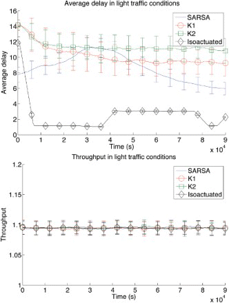
Figure 5. Average delay and throughput for a light traffic level (10 cars spawned per minute at each entrance). Error bars show one standard deviation.

Figure 6. Average delay and throughput for a heavy traffic level (30 cars spawned per minute at each entrance). Error bars show one standard deviation.
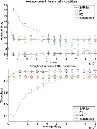
Figure 6. Average delay and throughput for a heavy traffic level (30 cars spawned per minute at each entrance). Error bars show one standard deviation.

Figure 7. The reward samples observed during a single run with a heavy traffic level and either delay (a) or throughput (b) as a reward signal. Colour indicates the timing of the sample, with blue early in the run, and red at the end of the run. The objectives (minimising delay on x-axis and maximising throughput on y-axis) are observed to be correlated.
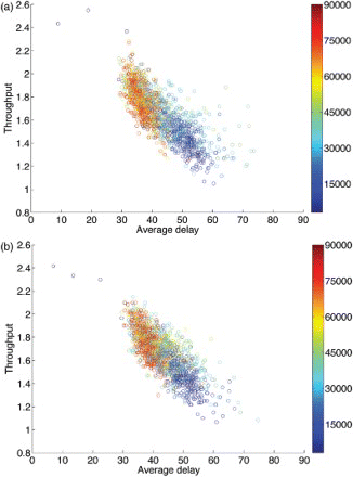
Figure 7. The reward samples observed during a single run with a heavy traffic level and either delay (a) or throughput (b) as a reward signal. Colour indicates the timing of the sample, with blue early in the run, and red at the end of the run. The objectives (minimising delay on x-axis and maximising throughput on y-axis) are observed to be correlated.

Figure 8. Average delay for a light traffic level (10 cars spawned per minute at each entrance). Comparison of two single-objective approaches and linear scalarisation. Error bars show one standard deviation.
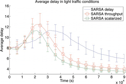
Figure 8. Average delay for a light traffic level (10 cars spawned per minute at each entrance). Comparison of two single-objective approaches and linear scalarisation. Error bars show one standard deviation.
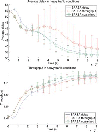
Figure 9. Average delay and throughput for a heavy traffic level (30 cars spawned per minute at each entrance). Comparison of two single-objective approaches and linear scalarisation. Error bars show one standard deviation.

Figure 9. Average delay and throughput for a heavy traffic level (30 cars spawned per minute at each entrance). Comparison of two single-objective approaches and linear scalarisation. Error bars show one standard deviation.

Figure 10. Average delay for a light traffic level (10 cars spawned per minute at each entrance). Comparison of delay, scalarised (delay and throughput), delay-squared and a different scalarised (delay squared and throughput) reward signal. Error bars show one standard deviation.
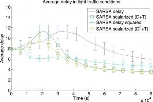
Figure 10. Average delay for a light traffic level (10 cars spawned per minute at each entrance). Comparison of delay, scalarised (delay and throughput), delay-squared and a different scalarised (delay squared and throughput) reward signal. Error bars show one standard deviation.

Figure 11. Average delay and throughput for a heavy traffic level (30 cars spawned per minute at each entrance). Comparison of delay, scalarised (delay and throughput) and delay-squared reward signals. Scalarised with delay-squared and throughput yields the same performance as delay-squared alone. Error bars show one standard deviation.
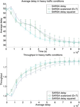
Figure 11. Average delay and throughput for a heavy traffic level (30 cars spawned per minute at each entrance). Comparison of delay, scalarised (delay and throughput) and delay-squared reward signals. Scalarised with delay-squared and throughput yields the same performance as delay-squared alone. Error bars show one standard deviation.

Reprints and Corporate Permissions

Please note: Selecting permissions does not provide access to the full text of the article, please see our help page How do I view content?

To request a reprint or corporate permissions for this article, please click on the relevant link below:

Academic Permissions

Please note: Selecting permissions does not provide access to the full text of the article, please see our help page How do I view content?

Obtain permissions instantly via Rightslink by clicking on the button below:

If you are unable to obtain permissions via Rightslink, please complete and submit this Permissions form. For more information, please visit our Permissions help page.