Towards Malay named entity recognition: an open-source dataset and a multi-task framework

Figures & data

Table 1. Malay NER datasets.

Datasets	Sen Num	Tok Num	Entity type	Data source
Asmai et al. (2018)	17,527	/	5	Crime
Salleh et al. (2017)	/	/	4	News
Ulanganathan et al. (2017)	/	275,322	4	/
Zamin and Bakar (2015)	/	16,061	3	News
Zamin et al. (2013)	263	5413	3	News

Table 2. Data source.

Website	URL
Bharian	http://www.bharian.com.my/
Utusan	http://www.utusan.com.my/
Malaysiakini	http://www.malaysiakini.com/bm

Figure 1. Dataset construction process. It consists of two parts: preliminary construction and iterative optimisation.

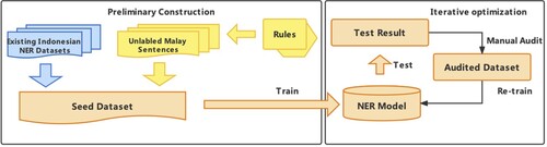
Table 3. Audit guideline.

Entity	Guideline	Example
Person	Include punctuation in the middle of names.	Edry D'putra Hayadi
	Fictional characters referred to by name are included.	Latif Purnama
	Pronouns, reflexive pronouns, name prefixes are not included.	Mr., You, Me
Location	Include punctuation in the middle of names.	Madinat al-Zahra
	Fictional locations referred to by name are included.	Negara Terbang
	Geopolitical entities (such as city, state, country, continent, etc.) are included.	Kuala Lumpur
	Generic references are not included.	lapangan terbang
Organization	Include punctuation in the middle of names.	Al-Qaeda
	Fictional organisations referred to by name are included.	Tentera Udara Diraja Terbang
	Products or branches are not included.	Ghee Hiang
O	Tokens that do not belong to person, location, and organisation are included.	ketika

Table 4. An example of MS-NER.

Token	Label
Namun	O
,	O
satu	O
insiden	O
berlaku	O
di	O
Lapangan	B-LOC
Terbang	I-LOC
Incheon	I-LOC
menemukan	O
Bella	B-PER
dengan	O
seorang	O
lelaki	O
kacukan	O
Korea	B-LOC
iaitu	O
Danial	B-PER
Lee	I-PER
Jae	I-PER
Hwan	I-PER
.	O

Figure 2. The MTBR framework structure. Due to space limitation, [B-P, I-P, B-L, I-L, B-O, I-O, O] in the figure represents [B-PER, I-PER, B-LOC, I-LOC, B-ORG, I-ORG, OTHER].

Figure 3. Probability alignment. If $w_i$ is the first token of the detected entity, the probabilities would flow towards the black arrow; otherwise they would flow towards the red arrow.

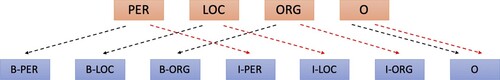
Table 5. Model settings.

Model	Component	Parameter	Value
Neural components	CNN	Filter size	3
		Number of filters	30
	Bi-LSTM	Number of units	200
	Optimizer	Optimizer function	SGD
		Learning rate	0.01
	Word embedding	Word embedding	GloVe
		Dimension	300
ELMO	Optimizer	Optimizer function	SGD
		Learning Rate	0.015
		Learning Rate Decay	0.05
BERT	Optimizer	Optimizer function	Adam
		Learning rate	5e−5
		Weight decay	0.001
–	Common Max length	128
		Data source	News

Table 6. Main performance.

Framework	Method	P (%)	R (%)	F1 (%)
Single-task Model	NeuralNER	88.66	87.31	87.98
	Bi-LSTM-CNNs	89.01	87.72	88.36
	Bi-LSTM-CNNs-CRF	88.73	88.12	88.42
	ELMO-softmax	91.12	89.67	90.39
	mBERT-softmax	91.02	89.55	90.28
	Bahasa-BERT-softmax	91.01	90.11	90.56
	Bahasa-BERT-CRF	90.89	91.22	91.05
	Bahasa-BERT-MRC	91.33	91.02	91.17
Multi-task model	Bi-LSTM-PN	88.25	88.46	88.36
	MT-MED	89.57	88.85	89.20
	MT-BERT	91.80	90.24	91.01
	MTBR (CNNs-Bi-LSTM)	89.91	89.69	89.80
	MTBR (ELMO)	92.97	91.44	92.20
	MTBR (Bahasa-BERT)	92.70	92.01	92.36

Note: • mBERT(https://huggingface.co/bert-base-multilingual-cased)

Table 7. Performance of different modules.

Model	P (%)	R (%)	F1 (%)
w/o Boundary detection	91.01	90.11	90.56
w/o Bi-Revision	91.80	90.24	91.01
w/o Gated ignoring mechanism	92.70	90.89	91.79
w/o Random probability	92.66	91.34	92.00
MTBR	92.70	92.01	92.36

Table 8. BRE analysis.

Model	BRE (%)
Sigle-task Model	3.53
Standard Multi-task model	2.79
MTBR	1.89

Table 9. Case study. MTBR gives all correct predictions in these cases.

Example1	Glyn Davies kerana kritikan yang dibuatkannya pada satu majlis di Kelab Wartawan Asing Thailand. (Glyn Davies for the criticism he made at an event at the Thai Foreign Journalists Club.)
BD module	Glyn Davies: [PER], Kelab Wartawan Asing Thailand: [ORG]
NER module	Glyn Davies: [PER], Kelab Wartawan Asing: [ORG], Thailand: [LOC]
MTBR	Glyn Davies: [PER], Kelab Wartawan Asing Thailand: [ORG]
Example2	Ketua Setiausaha Perbendaharaan, Tan Sri Dr Mohd Irwan Seregar Abdullah, (Chief Secretary of the Treasury, Tan Sri Dr Mohd Irwan Seregar Abdullah,)
BD module	Tan Sri Dr Mohd Irwan Seregar Abdullah: [PER]
NER module	Tan Sri: [PER], Dr Mohd Irwan Seregar: [PER]
MTBR	Tan Sri Dr Mohd Irwan Seregar Abdullah: [PER]
Example3	Brahim's Dewina dengan kerjasama Baitul Hayati pula akan mengumpul dan mengagihkan makanan berkenaan setiap hari termasuk memasak serta membungkuskannya. (Brahim's Dewina in collaboration with Baitul Hayati will collect and distribute the food every day including cooking and packing it.)
BD module	Brahim's Dewina: [PER], Baitul Hayati: [PER]
NER module	Brahim's Dewina: [ORG], Baitul Hayati: [ORG]
MTBR	Brahim's Dewina: [ORG], Baitul Hayati: [ORG]

Table 10. MTBR performance on more languages.

Framework	Method	en	id
Single-task Model	NeuralNER	90.94	86.94
	Bi-LSTM-CNNs	91.62	87.44
	Bi-LSTM-CNNs-CRF	91.21	87.84
	ELMO-softmax	92.20	88.71
	BERT-softmax	92.40	88.61
	BERT-CRF	92.60	88.50
	BERT-MRC	93.03	90.02
Multi-task Model	Bi-LSTM-PN	90.32	85.43
	MT-MED	92.01	86.34
	MT-BERT	92.89	90.38
	MTBR (CNNs-Bi-LSTM)	92.09	89.02
	MTBR (ELMO)	92.99	90.87
	MTBR (BERT)	93.36	91.13

Asmai, S. A., Salleh, M. S., Basiron, H., & Ahmad, S. (2018). An enhanced Malay named entity recognition using combination approach for crime textual data analysis. International Journal of Advanced Computer Science and Applications, 9(9). https://doi.org/10.14569/issn.2156-5570

 Google Scholar

Salleh, M. S., Asmai, S. A., Basiron, H., & Ahmad, S. (2017). A Malay named entity recognition using conditional random fields. In 2017 5th international conference on information and communication technology (ICOIC7) (pp. 1–6). IEEE. https://doi.org/10.1109/ICoICT.2017.8074647.

 Google Scholar

Ulanganathan, T., Ebrahim, A., Xian, B. C. M., Bouzekri, K., Mahmud, R., & Hoe, O. H. (2017). Benchmarking Mi-NER: Malay entity recognition engine. In 9th international conference on information, process, and knowledge management (pp. 52–58).

 Google Scholar

Zamin, N., & Bakar, Z. A. (2015). Name entity recognition for malay texts using cross-lingual annotation projection approach. In O. Gervasi (Eds.), Computational science and its applications – ICCSA 2015 – 15th international conference proceedings, part I, June 22–25 (Vol. 9155, pp. 242–256). Springer. https://doi.org/10.1007/978-3-319-21404-7_18.

 Google Scholar

Zamin, N., Oxley, A., & Bakar, Z. A. (2013). Projecting named entity tags from a resource rich language to a resource poor language. Journal of Information and Communication Technology, 12, 121–146. https://e-journal.uum.edu.my/index.php/jict/article/view/8140.

 Google Scholar