ZigZag transform with Durstenfeld shuffle for fast and secure image encryption

Figures & data

Figure 1. Classical ZigZag transform.

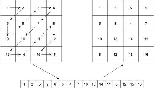
Figure 2. Improved ZigZag transform with Durstenfeld shuffle algorithm.

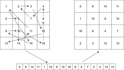
Figure 3. System architecture of the proposed encryption process.

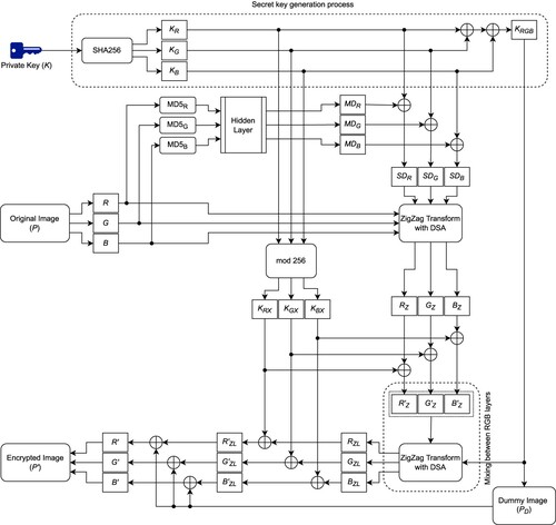
Figure 4. Key generation for RGB channels from the SHA256 hash of private key.

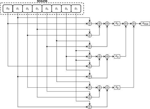
Table 1. Guiding information to select pairs of blocks to XOR.

Input								Output
$D_0$	$D_1$	$D_2$	$D_3$	$D_4$	$D_5$	$D_6$	$D_7$	$K_R$	$K_G$	$K_B$
1	1	0	0	0	0	0	0	$K_{R_1}$	0	0
0	0	1	1	0	0	0	0	$K_{R_2}$	0	0
0	0	0	0	1	1	0	0	$K_{R_3}$	0	0
0	0	0	0	0	0	1	1	0	$K_{G_1}$	0
1	0	0	0	0	0	0	1	0	$K_{G_2}$	0
0	1	0	0	0	0	1	0	0	$K_{G_3}$	0
0	0	1	0	0	1	0	0	0	0	$K_{B_1}$
0	0	0	1	1	0	0	0	0	0	$K_{B_2}$
0	1	0	0	0	0	0	1	0	0	$K_{B_3}$

Figure 5. Hidden key generation for RGB using MD5 hashing (one of the possible configurations).

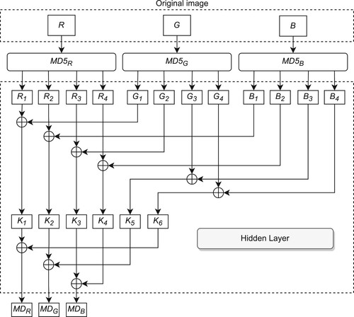
Figure 6. Experimental results for encryption and decryption, (a)–(d) plaintext images Lena, Pepper, Baboon and Barbara, (e)–(h) encrypted images Lena, Pepper, Baboon and Barbara, (i)–(l) decrypted images Lena, Pepper, Baboon and Barbara.

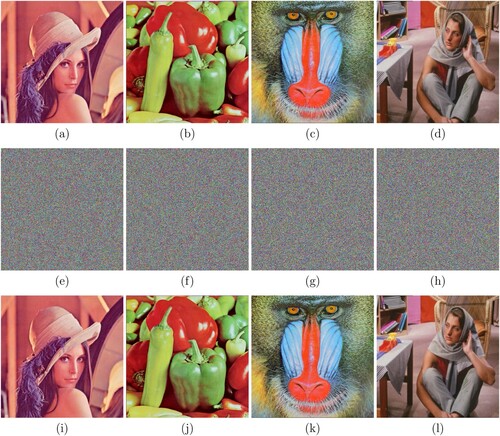
Figure 7. Experimental results for encryption and decryption with all white and all black images.

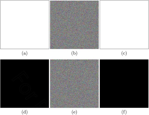
Figure 8. Decryption results with correct and incorrect keys: (a) decrypted image with the correct key maltepe@, (b)–(f) images decrypted with keys with little difference (Maltepe@, malTepe@, ma1ltepe, maltrpe_, maltePe).

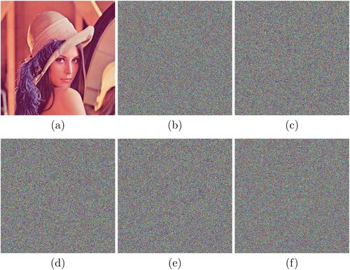
Table 2. NPCR (%) values of decrypted images with different keys.

Channels	(a)	(b)	(c)	(d)	(e)	(f)
R	0	99.60	99.60	99.60	99.59	99.62
G	0	99.58	99.60	99.61	99.62	99.62
B	0	99.61	99.63	99.62	99.61	99.60

Figure 9. Histogram analysis: (a) histogram of the plaintext Lena in all channels, (b)–(d) histograms of the ciphertext image Lena in channels R, G and B, respectively, (e) histogram of the plaintext Pepper in all channels, (f)–(h) histograms of the ciphertext image Pepper in channels R, G and B, respectively, (i) histogram of the plaintext Baboon in all channels, (j)–(l) histograms of the ciphertext image Baboon in channels R, G and B, respectively, (m) histogram of the plaintext Barbara in all channels, (n)–(p) histograms of the ciphertext image Barbara in channels R, G and B, respectively.

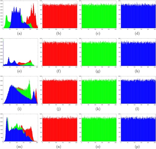
Figure 10. Correlation between adjacent pixels in channel R of Lena: (a)–(c) horizontal, vertical and diagonal correlations in plaintext, (d)–(f) horizontal, vertical, diagonal correlations in ciphertext.

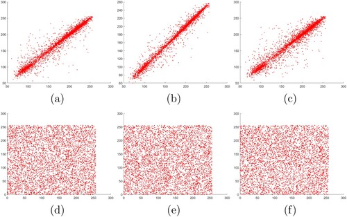
Figure 11. Correlation between adjacent pixels in channel G of Lena: (a)–(c) Horizontal, vertical, and diagonal correlations in plaintext, (d)–(f) horizontal, vertical, diagonal correlations in ciphertext.

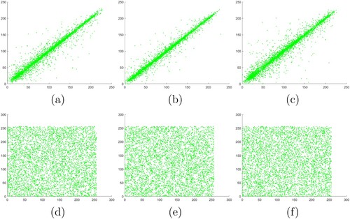
Figure 12. Correlation between adjacent pixels in channel B of Lena: (a)–(c) horizontal, vertical and diagonal correlations in plaintext, (d)–(f) horizontal, vertical, diagonal correlations in ciphertext.

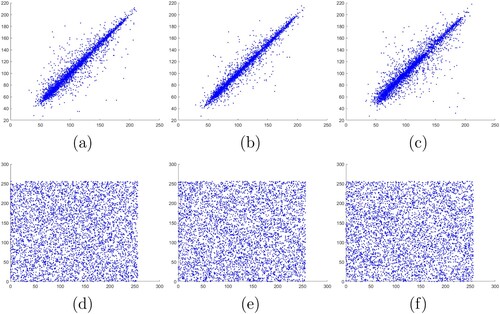
Table 3. Correlations between adjacent pixels of plaintext and ciphertext images of Lena.

	Horizontal			Vertical			Diagonal
Method	R	G	B	R	G	B	R	G	B
Plaintext	0.9783	0.9787	0.9593	0.9896	0.9900	0.9791	0.9675	0.9686	0.9409
Our Method	0.0008	−0.0005	−0.0032	0.0026	0.0010	0.0009	0.0007	−0.0003	−0.0014
Xingyuan et al. (2019)	−0.3131	−0.0007	0.0036	0.0142	−0.0167	0.0083	−0.0044	−0.0145	−0.0214
Ben Slimane et al. (2018)	0.0271	0.0021	0.0205	0.0297	0.0168	0.0029	0.0254	0.0011	0.0172
Gan et al. (2018)	−0.0084	−0.0077	−0.0232	−0.0134	0.0237	0.0063	0.0059	0.0085	0.0176
Arpacı et al. (2020)	−0.0125	0.0184	0.0096	0.0118	0.0221	0.0030	0.0009	−0.0041	−0.0009
Yang and Chien (2020)	−0.0003	0.0012	−0.0038	−0.0012	−0.0009	−0.0007	−0.0005	−0.0038	0.0029
Chai et al. (2020)	0.0027	−0.0167	0.0033	−0.0124	0.0153	−0.0004	0.0022	−0.0127	−0.0027
Firdous and Missen (2019)	0.0105	0.0073	−0.0134	−0.0391	0.0114	−0.0312	0.0028	−0.0081	−0.0184

Table 4. Entropy analysis results (in bits).

Test image	R	G	B
Plaintext Lena	7.2584	7.5791	6.9810
Ciphertext Lena	7.9993	7.9994	7.9993
Ben Slimane et al. (2018)	7.9984	7.9981	7.9977
Gan et al. (2018)	7.9993	7.9992	7.9994
Arpacı et al. (2020)	7.9995	7.9988	7.9991
Chai et al. (2020)	7.9995	7.9993	7.9992
Firdous and Missen (2019)	7.9993	7.9992	7.9992

Table 5. NPCR and UACI values of ciphertext images of Lena for plaintext sensitivity analysis.

	NPCR (%)			UACI (%)
Method	R	G	B	R	G	B
Our method	99.61	99.61	99.62	33.33	33.41	33.42
Ben Slimane et al. (2018)	99.63	99.62	99.61	33.46	33.45	33.45
Gan et al. (2018)	99.61	99.60	99.59	33.47	33.42	33.48
Arpacı et al. (2020)	99.60	99.61	99.59	33.49	33.44	33.49
Firdous and Missen (2019)	99.58	99.61	99.65	33.45	33.49	33.44
Devaraj and Kavitha (2016)	99.61	99.79	99.79	38.00	37.10	31.94
Zhang et al. (2020)	99.62	99.61	99.62	33.42	33.43	33.46

Figure 13. Experimental results for a noise attack. Gaussian noise decryption results with variance of (a) 0.01 and (b) 0.1. Salt-and-pepper noise decryption results with intensity of (c) 0.01 and (d) 0.05.

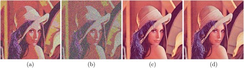
Figure 14. Experimental results for occlusion attacks. The encrypted images with (a) 1/16, (b) 1/4 and (c) 1/2 occlusion, (d) Plus occlusion, (e)–(h) are the corresponding decrypted images.

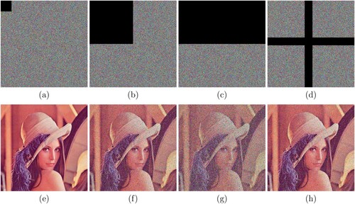
Table 6. Quantitative results of occlusion attack resistance.

	MSE			PSNR			NPCR (%)			UACI (%)
Occlusion	R	G	B	R	G	B	R	G	B	R	G	B
1/16	13.15	11.74	10.34	25.75	26.74	27.84	1.57	1.56	1.54	0.53	0.52	0.51
1/4	51.77	47.28	41.75	13.85	14.64	15.72	24.90	24.84	24.93	8.31	8.36	8.26
1/2	73.10	67.05	59.13	10.85	11.60	12.70	49.78	49.79	49.83	16.57	16.77	16.55
Plus	48.99	44.92	39.65	14.33	15.08	16.17	22.32	22.39	22.36	7.46	7.52	7.43

Table 7. NIST test results.

Test	P-value	Pass/Fail
Frequency test	0.888	Pass
Block frequency test	0.809	Pass
Cumulative sums test-forward	0.423	Pass
Cumulative sums test-reverse	0.867	Pass
Runs test	0.252	Pass
Longest run test	0.733	Pass
Discrete Fourier transform test	0.604	Pass
Rank test	0.903	Pass
Non overlapping template test	1.000	Pass
Overlapping template test	0.895	Pass
Universal test	0.995	Pass
Approximate entropy test	0.660	Pass
Serial test	0.522	Pass
Random excursions test	0.594	Pass
Random excursions variant test	0.317	Pass
Linear complexity test	0.454	Pass

Xingyuan, W., Junjian, Z., & Guanghui, C. (2019). An image encryption algorithm based on ZigZag transform and LL compound chaotic system. Optics & Laser Technology, 119, Article ID 105581. https://doi.org/10.1016/j.optlastec.2019.105581.

 Web of Science ®Google Scholar

Ben Slimane, N., Aouf, N., Bouallegue, K., & Machhout, M. (2018). A novel chaotic image cryptosystem based on DNA sequence operations and single neuron model. Multimedia Tools and Applications, 77(23), 30993–31019. https://doi.org/10.1007/s11042-018-6145-8.

 Web of Science ®Google Scholar

Gan, Z., Chai, X., Zhang, M., & Lu, Y. (2018). A double color image encryption scheme based on three-dimensional Brownian motion. Multimedia Tools and Applications, 77(21), 27919–27953. https://doi.org/10.1007/s11042-018-5974-9.

 Web of Science ®Google Scholar

Arpacı, B., Kurt, E., Çelik, K., & Ciylan, B. (2020). Colored image encryption and decryption with a new algorithm and a hyperchaotic electrical circuit. Journal of Electrical Engineering & Technology, 15(3), 1413–1429. https://doi.org/10.1007/s42835-020-00393-x.

 Web of Science ®Google Scholar

Yang, C. H., & Chien, Y. S. (2020). FPGA implementation and design of a hybrid chaos-AES color image encryption algorithm. Symmetry, 12(2), 189. https://doi.org/10.3390/sym12020189.

 Google Scholar

Chai, X., Zheng, X., Gan, Z., & Chen, Y. (2020). Exploiting plaintext-related mechanism for secure color image encryption. Neural Computing and Applications, 32(12), 8065–8088. https://doi.org/10.1007/s00521-019-04312-8.

 Web of Science ®Google Scholar

Firdous, A., & Missen, M. M. S. (2019). A highly efficient color image encryption based on linear transformation using chaos theory and SHA-2. Multimedia Tools and Applications, 78(17), 24809–24835. https://doi.org/10.1007/s11042-019-7623-3.

 Web of Science ®Google Scholar

Devaraj, P., & Kavitha, C. (2016). An image encryption scheme using dynamic S-boxes. Nonlinear Dynamics, 86(2), 927–940. https://doi.org/10.1007/s11071-016-2934-7.

 Web of Science ®Google Scholar

Zhang, Y. Q., He, Y., Li, P., & Wang, X. Y. (2020). A new color image encryption scheme based on 2DNLCML system and genetic operations. Optics and Lasers in Engineering, 128, Article ID 106040. https://doi.org/10.1016/j.optlaseng.2020.106040.

 Web of Science ®Google Scholar